PCA III#
Download#
How many principal components is “enough”?#
#| echo: true
library(pdfCluster)
data(oliveoil)
OO = oliveoil[,3:10]
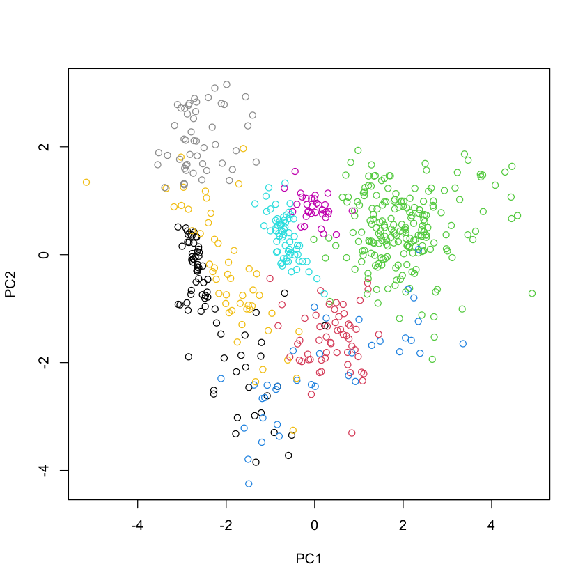
pcaOO = prcomp(OO, scale.=TRUE)$x
plot(pcaOO, col=oliveoil$region)
pdfCluster 1.0-4
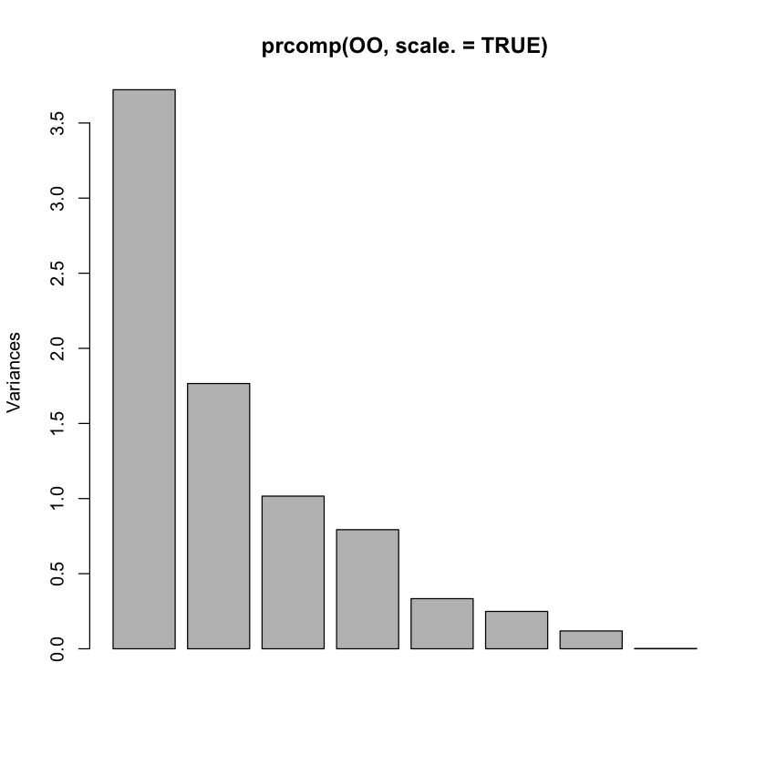
Is there an elbow?#
plot(prcomp(OO, scale.=TRUE))
Is there an elbow? Tuzhilina, Hastie & Segal (2022)#
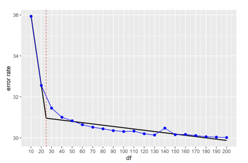
Do we need to pick a rank?#
Visualization#
Many applied settings use PCA simply to visualize the data.
For this, typically only the first few PCs are used. No need to really pick a rank…
Testing#
Suppose we believe \(X \sim N(0, I \otimes \Sigma)\).
If we think \(\Sigma = \sigma^2 I + VV^T\) then we might want to decide if \(V=0\) or not… what rank is \(V\)?
Note: \(\text{rank}(V)\) is not the rank of \(\Sigma\)…
Do we need to pick a rank?#
Modeling#
The matrix \(X\) may show up later in downstream analyses using its PCs for regression. \(\implies\) can use CV to pick ranks. number of PCs.
We may want to fit a generative model to \(X\) itself: probabilistic PCA of Bishop & Tittering (1999)
Estimation#
Suppose we believe \(X \sim N(\mu, I \otimes I)\) and want to estimate \(\mu\) by hard-thresholding the singular values
How do we pick \(c\)?
Testing#
Classical theory#
Suppose \(X_{n \times p} \sim N(0, I_{n \times n} \otimes \Sigma)\)
Often (e.g. as presented in MKB) assumes \(n \to \infty\) and \(p\) essentially fixed.
Allows (with extra conditions) for MLE analysis of eigendecomposition of \(\Sigma=U\Lambda U^T\)
Notes there is ambiguity when there are ties in \(\Lambda\): variance of MLE of \(U[,i]\) depends on gaps \(\lambda_{i-1}-\lambda_i\) and \(\lambda_i - \lambda_{i+1}\)…
Could it be used for testing \(H_0:\Sigma=\sigma^2 \cdot I\) vs. \(H_a:\Sigma=\sigma^2 \cdot I + vv^T\) for \(v \in \mathbb{R}^p\)? (wlog \(\sigma^2=1\) going forward)
We know LRT here would be based on \(\log \det(\hat{\Sigma})\).
As all gaps are 0 under the null, at face value this is a context where much of \(\Sigma\) is poorly estimable…
Largest eigenvalue#
Maybe better motivated to use largest eigenvalue
How do eigenvalues behave under \(H_0\), particularly with \(n, p\) comparable?
Eigenvalues of large Wishart matrices#
Set \(p/n=\gamma\) and consider the eigenvalues of \(X \sim N(0, I_{n \times n} \otimes I_{p \times p})\).
The population eigenvalues of \(\mathbb{E}[\Sigma]\) are all (essentially) 1…
What about the sample eigenvalues?
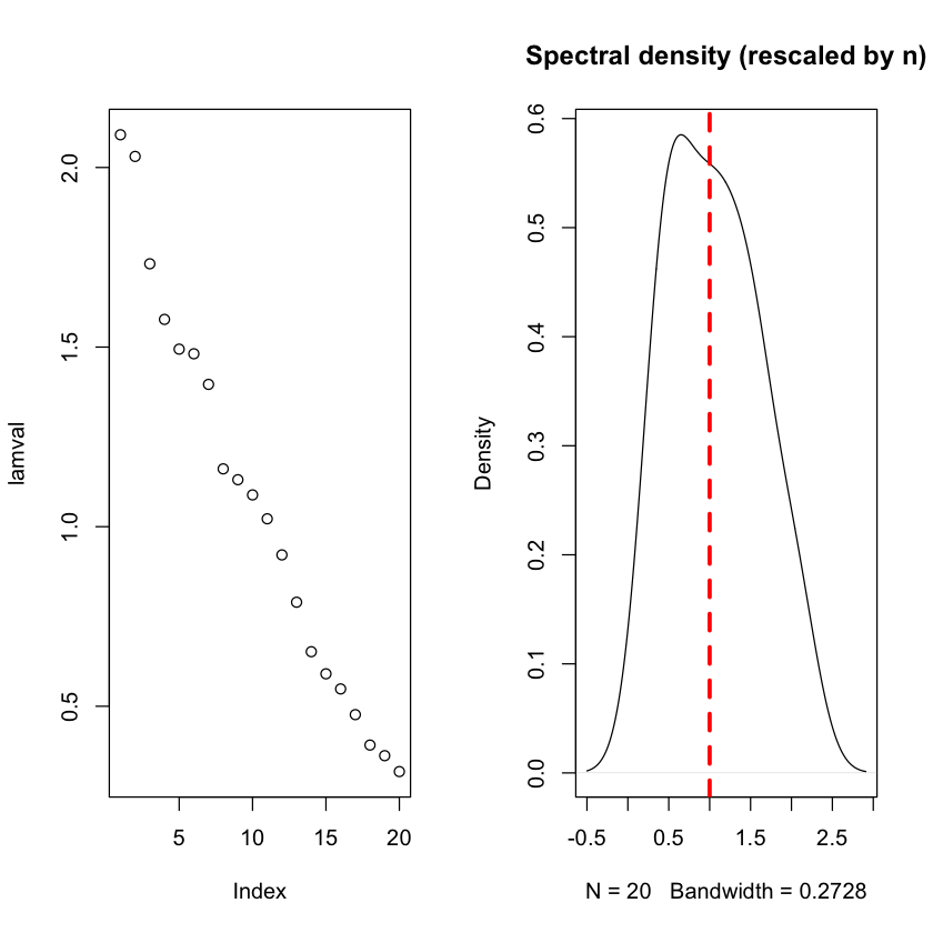
Eigenvalues of large-ish Wishart matrices \(n=80, p=20\)#
#| echo: false
n = 80
p = 20
X = matrix(rnorm(n * p), n, p)
lamval = svd(X)$d^2 / n
par(mfrow=c(1,2))
plot(lamval)
plot(density(lamval), main='Spectral density (rescaled by n)')
abline(v=1, lwd=3, lty=2, col='red')
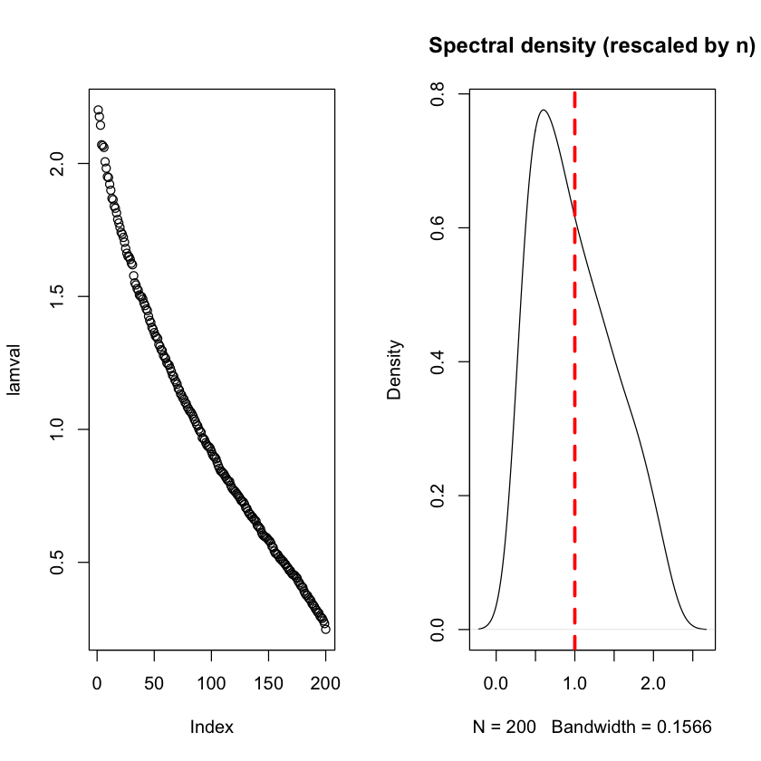
Eigenvalues of large-ish Wishart matrices \(n=800, p=200\)#
#| echo: false
n = 800
p = 200
X = matrix(rnorm(n * p), n, p)
lamval = svd(X)$d^2 / n
par(mfrow=c(1,2))
plot(lamval)
plot(density(lamval), main='Spectral density (rescaled by n)')
abline(v=1, lwd=3, lty=2, col='red')
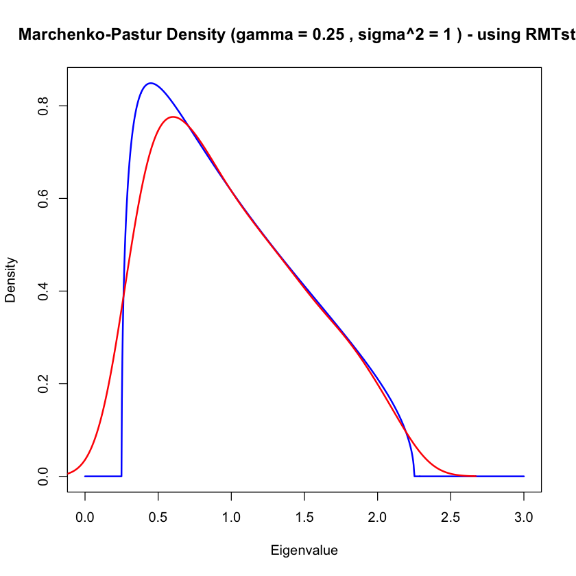
Marchenko-Pastur \(\gamma=1/4\)#
#| echo: false
library(RMTstat)
curve(dmp(x, svr = n/p, var = 1),
      from = 0, to = 3,
      n = 1000,
      col = "blue",
      lwd = 2,
      ylab = "Density",
      xlab = "Eigenvalue",
      main = paste("Marchenko-Pastur Density (gamma =", p/n, ", sigma^2 =", 1, ") - using RMTstat"))
lines(density(lamval), col='red', lwd=2)
Marchenko-Pastur#
With \(W \sim \text{Wishart}(n, I_{p \times p})\) M&P derived the (limiting) density of the spectral measure
With \(\gamma=p/n\) the support is \((1 \pm \sqrt{\gamma})^2\) so if \(\gamma > 0\) then there is spread around the “population” spectrum \(\delta_1\)…
Baik-Ben Arous-Peche#
For \(H_a: \Sigma = I + vv^T\) unless \(1 + \|v\|^2 > (1 + \sqrt{\gamma})^2\) the perturbed eigenvalue will not be visible in this limiting spectrum…
Largest eigenvalue#
\(\implies\) for testing, we might look at the behavior near \((1 + \sqrt{\gamma})^2\)…
Tracy-Widom and PCA#
Johnstone (2001) derived limiting law under \(H_0\):
Scaling and centering \((\sigma^2=1)\)#
Example#
#| echo: true
library(RMTstat)
X = matrix(rnorm(500), 50, 10)
eigvals_hat = svd(X)$d^2 / (nrow(X) - 1)
P_c = diag(rep(1, 50)) - matrix(1, 50, 50) / 50
Sigma_hat = t(X) %*% P_c %*% X / (nrow(X) - 1)
noise_level = sum(diag(Sigma_hat)) / ncol(X)
pWishartMax(eigvals_hat[1], nrow(X) - 1, ncol(X), var=noise_level, lower.tail=FALSE)
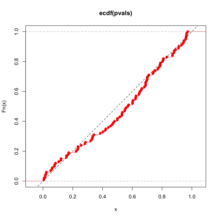
Run a few simulations \(n=50, p=10\)#
#| echo: false
simulate = function(n=50, p=10, nrep=100, which=1, delta=0) {
    pvals = c()
    P_c = diag(rep(1, n)) - matrix(1, n, n) / n
    for (b in 1:nrep) {
        X = matrix(rnorm(n*p), n, p)
        Sigma_hat = t(X) %*% P_c %*% X / (nrow(X) - 1)
        eigvals_hat = svd(P_c %*% X)$d^2 / (nrow(X) - 1)
        noise_level = sum(eigvals_hat[(which+delta):length(eigvals_hat)]) / (ncol(X) - (which + delta))
        pval = pWishartMax(eigvals_hat[which], nrow(X) - 1, ncol(X) - which + delta,
                           var=noise_level, lower.tail=FALSE)
        pvals = c(pvals, pval)
    }
    return(pvals)
}
#| echo: true
pvals = simulate(n=50, p=10)
plot(ecdf(pvals), col='red')
abline(c(0, 1), lty=2)
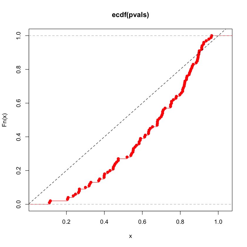
Run a few simulations \(n=300, p=200\)#
#| echo: true
pvals = simulate(n=300, p=200)
plot(ecdf(pvals), col='red')
abline(c(0, 1), lty=2)
Picking a rank#
Given a test statistic for the largest eigenvalue, there’s a natural “forward stepwise” procedure: starting at \(k=0\)
Compare \(d_{k+1}\) to appropriate quantile (\(1-\alpha\) ?) of Tracy-Widom (\(TW_1\)).
If larger, then \(k += 1\) and return to 1. Else stop.
Basis of pseudorank of Krichtman and Nadler (2008)
A little more refined (and involved) model Choi et al. (2017)
Estimation#
A different goal…#
Suppose now \(X \sim N(\mu, I \otimes I)\) and our goal is to recover \(\mu\)
Quality is to be judged by MSE:
In testing context, BPP phenomenon says only large enough (properly scaled) eigenvalues will surpass the edge \((1 + \sqrt{\gamma})^2\)
Suggests hard thresholding eigenvalues at \((1 + \sqrt{\gamma})^2\): a formal elbow rule….
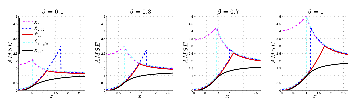
Optimal estimation#
Gavish and Donoho (2013) show that this choice is not asymptotically minimax optimal one in terms of MSE even if it can be used to properly determine the rank of \(V\) in \(H_a:I + VV'\)…
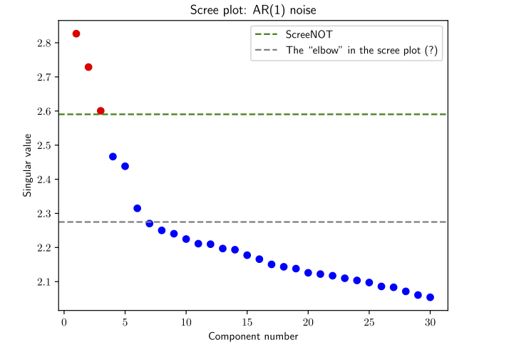
This work has been extended beyond standard Wishart in ScreeNOT (2022)
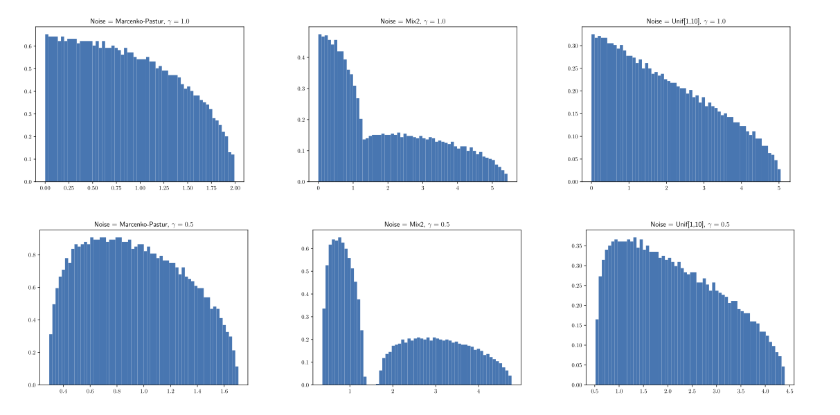
Rough approach: given the limiting spectrum of “noise”, they can derive an asymptotically optimal thresholding function.
Gavish and Donoho#
ScreeNOT#
ScreeNOT - noise spectra#
Probabilistic PCA#
Probabilistic PCA model#
We talked about models of the form \(I + VV'\) as alternatives in testing \(H_0:\Sigma=I\).
This model is essentially [Probabilistic PCA]: \(q < p\)
Makes assumption that the noise in \(X\) are all on the same scale… scaling \(X\) doesn’t magically fix this…
What PPCA gives us#
It models a low-rank structure within the covariance, not as the the covariance.
It gives us a likelihood, this allows:
AIC / BIC / CV for rank selection
Mixtures, Bayesian modeling etc (at least in theory)
Latent scores \(Z|X=x\)
Rank \(k\) MLE \(n > p\)#
Let \(\hat{\Sigma}_{MLE} = U D U'\).
Then, estimate \(\sigma^2\) as
To estimate \(V\), deflate by \(\sigma^2\):
where \(R_{k \times k}\) is an arbitrary rotation.
PPCA via EM#
Complete (negative) log-likelihood#
Note that \(Z|X \sim N\left(V'(VV' + \sigma^2 I)^{-1} X, I - V'(VV' + \sigma^2 I)^{-1}V\right)\)
Expected value given \(X\) at \((V_{\text{cur}}, \sigma^2_{\text{cur}}) = (V_c, \sigma^2_c)\) (ignoring irrelevant terms)#
Estimation of new \((V_{\text{new}}, \sigma^2_{\text{new}})\): multi response regression with covariance \(I_{n \times n} \otimes (\sigma^2 I_{p \times p})\)…
Example#
library(Rdimtools)
OOs = scale(OO)
ppcaOO = do.ppca(OOs, ndim=2)
plot(ppcaOO$Y[,1], ppcaOO$Y[,2], col=oliveoil$region)
print(ppcaOO$mle.sigma2)
# AIC(ppcaOO) # this fails unfortunately
** ------------------------------------------------------- **
** Rdimtools || Dimension Reduction and Estimation Toolbox
**
** Version : 1.1.2 (2025)
** Maintainer : Kisung You (kisungyou@outlook.com)
** Website : https://kisungyou.com/Rdimtools/
**
** Please see 'citation('Rdimtools)' to cite the package.
** ------------------------------------------------------- **
[1] 0.4187987
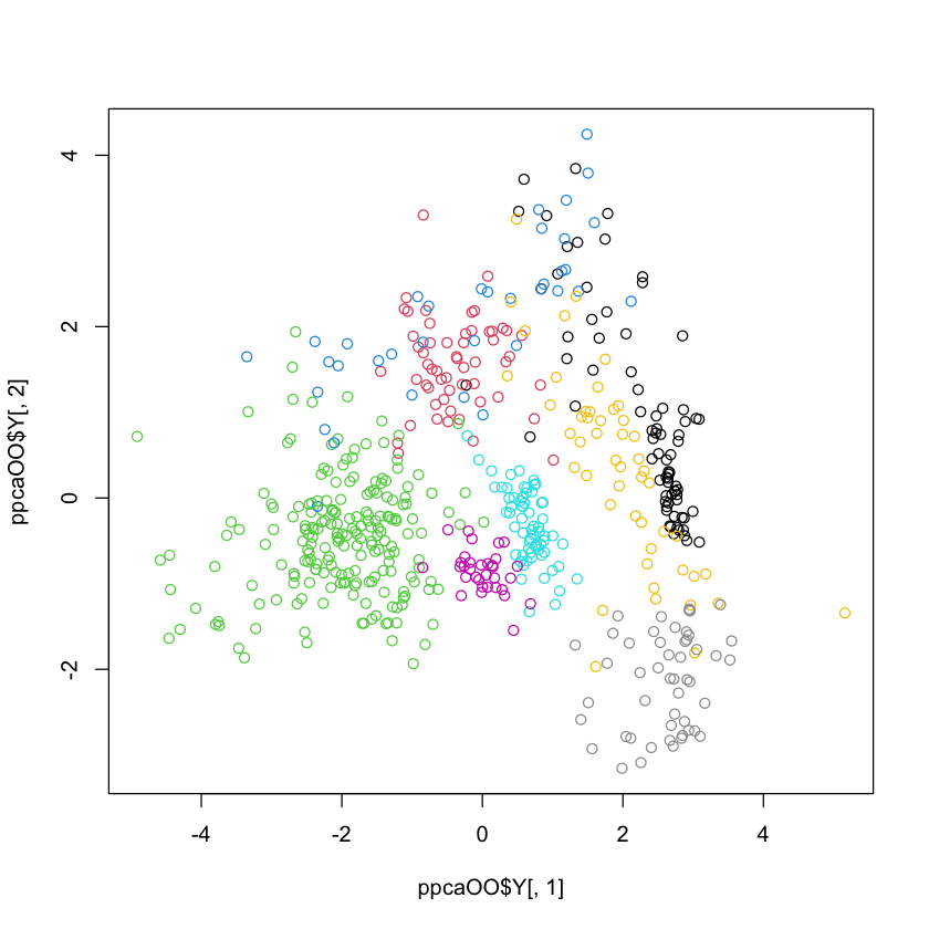
Did we gain much here?#
plot(pcaOO, col=oliveoil$region)