Assignment 3#
You may discuss homework problems with other students, but you have to prepare the written assignments yourself.
Please combine all your answers, the computer code and the figures into one file, and submit a copy in your dropbox on Gradescope.
Due date: 11:59 PM, May 10, 2024.
Grading scheme: 10 points per question, total of 40.
Building PDF#
If you have not installed LaTeX on your computer. After running the below commands (once is enough), then using either Quarto or RMarkdown formats should hopefully be sufficient to build directly to PDF.
install.packages('tinytex', repos='http://cloud.r-project.org')
tinytex::install_tinytex()
Download#
Question 1#
We revisit Tomasetti’s and Vogelstein’s study on cancer incidence across tissues from Assignment 2. The second part of their paper deals with the existence of two clusters in the dataset: According to the authors, D-tumours (D for deterministic) can be attributed to some degree to environmental and genetic factors, while the risk of R-tumours (R for replicative) is affected mainly by random mutations occuring during replication of stem cells.
Parts#
The dataset also includes a column
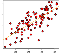
Clusteraccording to the classification of that tumour as Deterministic or Replicative. Fit a linear model as in Assignment 2, but with a different slope for D- and R-tumours.Make a scatterplot including the two regression lines.
Conduct a F-test to compare the regression model above to the regression model which does not account for this classification. What is the p-value?
Question 2#
Use the Carseats dataset from the packages ISLR2 for this problem
Parts#
Fit a multiple regression model to predict
SalesusingAdvertising,CompPrice,Price,UrbanandUS.Provide an interpretation of each coefficient in the model. Be careful – some of the variables in the model are categorical.
For which of the predictors can you reject the null hypothesis \(\beta_j=0\) at \(\alpha=0.05\)?
On the basis of the previous question, fit a smaller model that only uses the predictors for which there is evidence of association with the outcome.
How well do the models in parts 1. and 4. fit the data?
Using the model from part 4., obtain 90% confidence intervals for the coefficients.
Is there any evidence of outliers or high leverage observations in the model from part 4.?
Question 3#
The dataset state.x77 in R contains the following statistics (among
others) related to the 50 states in the USA:
Population: population estimate (1975)Income: per capita income (1974)Illiteracy: illiteracy (1970, percent of population)HS.Grad: percent high school graduates (1970)
Make it into a data frame using:
state.data = data.frame(state.x77)
We are interested in the relation between Income and the other 3 variables.
1. Produce a 4 by 4 scatter plot of the variables above.
2. Fit a multiple linear regression model to the data with Income as the
outcome and Population, Illiteracy, HS.Grad as the independent
variables.
For which of the predictors can you reject the null hypothesis \(\beta_j=0\) at \(\alpha=0.05\)?
Compare this model to the that uses only
Populationas a covariate.
5. Produce standard diagnostic plots of the multiple regression fit in part 2. Summarize the results.
6. Find states with outlying predictors by looking at the leverage values using hatvalues. Use
a cutoff of 0.2.
7. Find outliers, if any, in the response. Remove them from the data and refit a multiple linear regression model and compare the result with the previous fit.
Question 4#
The dataset iris in R gives the measurements in centimeters of the
variables sepal length and width and petal length and width, respectively, for
50 flowers from each of 3 species of iris.
data(iris)
Parts#
Fit a multiple linear regression model to the data with sepal length as the dependent variable and sepal width, petal length and petal width as the independent variables.
Test the reduced model of \(H_0: \beta_{\texttt sepal width}=\beta_{\texttt petal length} = 0\) with an F-test at level \(\alpha=0.05\)
Test \(H_0: \beta_{\texttt sepal width} = \beta_{\texttt petal length}\) at level \(\alpha=0.05\)
Test \(H_0: \beta_{\texttt sepal width} < \beta_{\texttt petal length}\) at level \(\alpha=0.05\).
