Bootstrap

Bootstrap#

Download#

Bootstrapping linear regression#

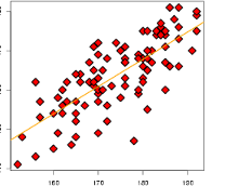
{height=400 fig-align=”center”}

Figure: our multiple linear regression model#

\[Y|X = X\beta + \epsilon\]

We’ve talked about checking assumptions.
What to do if the assumptions don’t hold?
We will use the bootstrap!

Random $X$: pairs bootstrap#

Suppose we think of the pairs $(X_i, Y_i)$ coming from some distribution $F$ – this is a distribution for both the features and the outcome.
In our usual model, $\beta$ is clearly defined. What is $\beta$ without this assumption?

Population least squares#

For our distribution $F$, we can define

\[ E_F[\pmb{X}\pmb{X}^T], \qquad E_F[\pmb{X} \cdot \pmb{Y}] \]

where $(\pmb{X}, \pmb{Y}) \sim F$ leading to

\[ \beta(F) = \left(E_F[\pmb{X}\pmb{X}^T]\right)^{-1} E_F[\pmb{X} \cdot \pmb{Y}]. \]

Asymptotics#

In fact, our least squares estimator is $\beta(\hat{F}_n)$ where $\hat{F}_n$ is the empirical distribution of our sample of $n$ observations from $F$.
As we take a larger and larger sample,

\[ \beta(\hat{F}_n) \to \beta(F) \]

and

\[ n^{1/2}(\beta(\hat{F}_n) - \beta(F)) \to N(0, \Sigma(F)) \]

for some covariance matrix $\Sigma=\Sigma(F)$ depending only on $F$.

Recall the variance of OLS estimator (with $X$ fixed): $$ (X^TX)^{-1} \text{Var}(X^T(Y-X\beta)) (X^TX)^{-1}. $$
With $X$ random and $n$ large this is approximately $$ \frac{1}{n} \left(E_F[\pmb{X}\pmb{X}^T] \right)^{-1} \text{Var}_F(\pmb{X} \cdot (\pmb{Y} - \pmb{X} \beta(F))) \left(E_F[\pmb{X}\pmb{X}^T] \right)^{-1}. $$

Population least squares#

In usual model,

\[\text{Var}(X^T(Y-X\beta)) = \sigma^2 X^TX \approx n \cdot E_F[\pmb{X} \pmb{X}^T].\]

This is wrong in general!
We will use OLS estimate – but correct its variance!
Can we get our hands on $\text{Var}(X^T(Y-X\beta))$ or $\text{Var}(\hat{\beta})$ without a model?

Nonparametric bootstrap in a nutshell#

Basic algorithm for pairs#

There are many variants of the bootstrap, most using roughly this structure

boot_sample = c()
for (b in 1:B) {
    idx_star = sample(1:n, n, replace=TRUE)
    X_star = X[idx_star,]
    Y_star = Y[idx_star]
    boot_sample = rbind(boot_sample, coef(lm(Y_star ~ X_star)))
}
cov_beta_boot = cov(boot_sample)

Residual bootstrap#

If $X$ is fixed, it doesn’t make sense to sample new $X$ values for $X^*$.
Residual bootstrap keeps $X$ fixed, but adds randomly sampled residuals

boot_sample = c()
M = lm(Y ~ X - 1)
beta.hat = coef(M)
X = model.matrix(M)
Y.hat = X @ beta.hat
r.hat = Y - Y.hat
for (b in 1:B) {
    idx_star = sample(1:n, n, replace=TRUE)
    X_star = X 
    Y_star = Y.hat + r.hat[idx_star]
    boot_sample = rbind(boot_sample, coef(lm(Y_star ~ X_star - 1)))
}
cov_beta_boot = cov(boot_sample)

Bootstrap for inference#

Estimated covariance cov_beta_boot can be used to estimate $\text{Var}(a^T\hat{\beta})$ for confidence intervals or general linear hypothesis tests.
Software does something slightly different – using percentiles of the bootstrap sample: bootstrap percentile intervals.

Bootstrapping regression#

Reference for more R examples #

library(car)
n = 50
X = rexp(n)
Y = 3 + 2.5 * X + X * (rexp(n) - 1) # our usual model is false here! 
Y.lm = lm(Y ~ X)

Loading required package: carData

pairs.Y.lm = Boot(Y.lm, coef, method='case', R=1000)
confint(Y.lm) 
confint(pairs.Y.lm, type='norm') # using bootstrap SE
confint(pairs.Y.lm, type='perc') # using percentiles

Loading required namespace: boot

A matrix: 2 × 2 of type dbl
	2.5 %	97.5 %
(Intercept)	2.501869	3.353018
X	2.235786	2.978521

A confint.boot: 2 × 2 of type dbl
	2.5 %	97.5 %
(Intercept)	2.626767	3.237522
X	2.021954	3.179938

A confint.boot: 2 × 2 of type dbl
	2.5 %	97.5 %
(Intercept)	2.565797	3.178609
X	2.135828	3.279040

Using the `boot` package#

The Boot function in car is a wrapper around the more general boot function.

library(boot)
D = data.frame(X, Y)
bootstrap_stat = function(D, bootstrap_idx) {
    return(summary(lm(Y ~ X, data=D[bootstrap_idx,]))$coef[,1])
}
boot_results = boot(D, bootstrap_stat, R=500)
confint(boot_results, type='norm') # using bootstrap SE
confint(boot_results, type='perc') # using percentiles

Attaching package: ‘boot’

The following object is masked from ‘package:car’:

    logit

A confint.boot: 2 × 2 of type dbl
2.5 %	97.5 %
2.613870	3.233349
2.021205	3.204503

A confint.boot: 2 × 2 of type dbl
2.5 %	97.5 %
2.556250	3.170863
2.110186	3.275172

How is the coverage?#

First we’ll use the standard regression model but errors that aren’t Gaussian.

noise = function(n) { return(rexp(n) - 1) }

simulate_correct = function(n=200, b=0.5) {
    X = rexp(n)
    Y = 3 + b * X + noise(n)
    Y.lm = lm(Y ~ X)

    # parametric interval
    int_param = confint(Y.lm)[2,]
    
    # pairs bootstrap interval   
    pairs.Y.lm = Boot(Y.lm, coef, method='case', R=500)
    pairs_SE = sqrt(cov(pairs.Y.lm$t)[2,2]) # $t is the bootstrap sample
    int_pairs = c(coef(Y.lm)[2] - qnorm(0.975) * pairs_SE,
                  coef(Y.lm)[2] + qnorm(0.975) * pairs_SE)

    result = c((int_param[1] < b) * (int_param[2] > b),
              (int_pairs[1] < b) * (int_pairs[2] > b))
    names(result) = c('parametric', 'bootstrap')
    return(result)
}

Check one instance#

simulate_correct()

parametric: 1
bootstrap: 1

Check coverage#

nsim = 100
coverage = c()
for (i in 1:nsim) {
    coverage = rbind(coverage, simulate_correct())
}
print(apply(coverage, 2, mean))

parametric  bootstrap 
      0.94       1.00 

Misspecified model#

Now we make data for which we might have used WLS but we don’t have a model for the weights!

simulate_incorrect = function(n=200, b=0.5) {
    X = rexp(n)
    # the usual model is 
    # quite off here -- Var(X^TY) is not well
    # approximated by sigma^2 * X^TX...
    Y = 3 + b * X + X * noise(n)
    Y.lm = lm(Y ~ X)

    # parametric interval
    int_param = confint(Y.lm)[2,]
    
    # pairs bootstrap interval
    pairs.Y.lm = Boot(Y.lm, coef, method='case', R=500)
    pairs_SE = sqrt(cov(pairs.Y.lm$t)[2,2]) # $t is the bootstrap sample of coefficients
                                            # we want the 2nd coefficient
    int_pairs = c(coef(Y.lm)[2] - qnorm(0.975) * pairs_SE,
                  coef(Y.lm)[2] + qnorm(0.975) * pairs_SE)

    result = c((int_param[1] < b) * (int_param[2] > b),
              (int_pairs[1] < b) * (int_pairs[2] > b))
    
    names(result) = c('parametric', 'bootstrap')
    return(result)
}

Check one instance#

simulate_incorrect()

parametric: 0
bootstrap: 0

Check coverage#

nsim = 100
coverage = c()
for (i in 1:nsim) {
    coverage = rbind(coverage, simulate_incorrect())
}

print(apply(coverage, 2, mean))

parametric  bootstrap 
      0.58       0.93 

Bootstrap

Contents

Bootstrap#

Download#

Bootstrapping linear regression#

Figure: our multiple linear regression model#

Random \(X\): pairs bootstrap#

Population least squares#

Asymptotics#

Population least squares#

Nonparametric bootstrap in a nutshell#

Basic algorithm for pairs#

Residual bootstrap#

Bootstrap for inference#

Bootstrapping regression#

Reference for more R examples #

Using the `boot` package#

How is the coverage?#

Check one instance#

Check coverage#

Misspecified model#

Check one instance#

Check coverage#

Bootstrap

Contents

Bootstrap#

Download#

Bootstrapping linear regression#

Figure: our multiple linear regression model#

Random \(X\): pairs bootstrap#

Population least squares#

Asymptotics#

Population least squares#

Nonparametric bootstrap in a nutshell#

Basic algorithm for pairs#

Residual bootstrap#

Bootstrap for inference#

Bootstrapping regression#

Reference for more R examples#

Using the boot package#

How is the coverage?#

Check one instance#

Check coverage#

Misspecified model#

Check one instance#

Check coverage#

Reference for more R examples #

Using the `boot` package#