Simple Linear Regression

Download

• Slides

• RStudio: RMarkdown,Quarto

• Jupyter

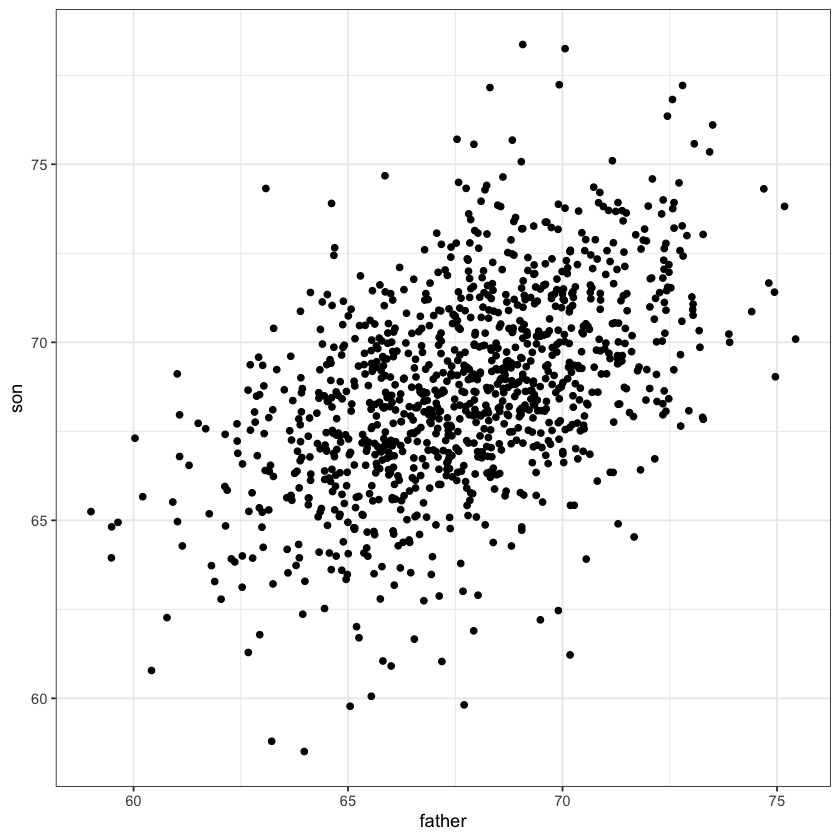
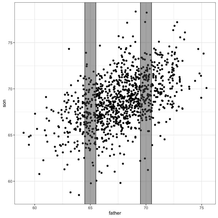
Father & son data

Pearson’s height data

library(UsingR)
heights = UsingR::father.son
head(heights)

Loading required package: MASS

Loading required package: HistData

Loading required package: Hmisc

Attaching package: ‘Hmisc’

The following objects are masked from ‘package:base’:

    format.pval, units

A data.frame: 6 × 2

	fheight	sheight
	<dbl>	<dbl>
1	65.04851	59.77827
2	63.25094	63.21404
3	64.95532	63.34242
4	65.75250	62.79238
5	61.13723	64.28113
6	63.02254	64.24221

# for scatter plots of heights
set.seed(1)
library(ggplot2)
library(UsingR)
heights = UsingR::father.son
heights$father = heights$fheight
heights$son = heights$sheight
height.lm = lm(son ~ father, data=heights)
intercept = height.lm$coef[1]
slope = height.lm$coef[2]

---

Father & son data

library(ggplot2)
heights_fig <- ggplot(heights, aes(father, son)) + geom_point() + theme_bw()
heights_fig

---

• An example of simple linear regression model.

• Breakdown of terms:

  1. regression model: a model for the mean of a response given features

  2. linear: model of the mean is linear in parameters of interest

  3. simple: only a single feature

---

Slicewise model

#| fig-align: center
rect = data.frame(xmin=69.5, xmax=70.5, ymin=-Inf, ymax=Inf)
heights_fig + geom_rect(data=rect, aes(xmin=xmin, xmax=xmax, ymin=ymin, ymax=ymax),
                        color="grey20",
                        alpha=0.5,
                        inherit.aes = FALSE)

• A simple linear regression model fits a line through the above scatter plot by modelling slices.

---

Conditional means

father = heights$fheight
son = heights$sheight
selected_points = (father <= 70.5) & (father >= 69.5)
mean(son[selected_points])

69.7684482608696

• The average height of sons whose height fell within our slice [69.5,79.5] is about 69.8 inches.

• This height varies by slice…

---

• At 65 inches it’s about 67.2 inches:

selected_points = (father <= 65.5) & (father >= 64.5)
mean(son[selected_points])

67.2231820792079

rect = data.frame(xmin=64.5, xmax=65.5, ymin=-Inf, ymax=Inf)
heights_fig + geom_rect(data=rect, aes(xmin=xmin, xmax=xmax, ymin=ymin, ymax=ymax),
                        color="grey20",
                        alpha=0.5,
                        inherit.aes = FALSE)

---

Multiple samples model (longevity example)

• We’ve seen this slicewise model before: error in each slice the same.

longevity = read.csv('https://raw.githubusercontent.com/StanfordStatistics/stats191-data/main/Sleuth3/longevity.csv', header=TRUE)
boxplot(Lifetime ~ Diet,
        data=longevity,
        col='orange',
        pch=23,
        bg='red')

---

Regression as slicewise model

• In longevity model: no relation between the means in each slice! We needed to use a parameter for each Diet…

• Regression model says that the mean in slice father is

\[ \beta_0+\beta_1 \cdot {\tt father}. \]

• This ties together all (father, son) points in the scatterplot.

• Chooses \((\beta_0, \beta_1)\) by jointly modeling the mean in each slice…

---

Height data as slices

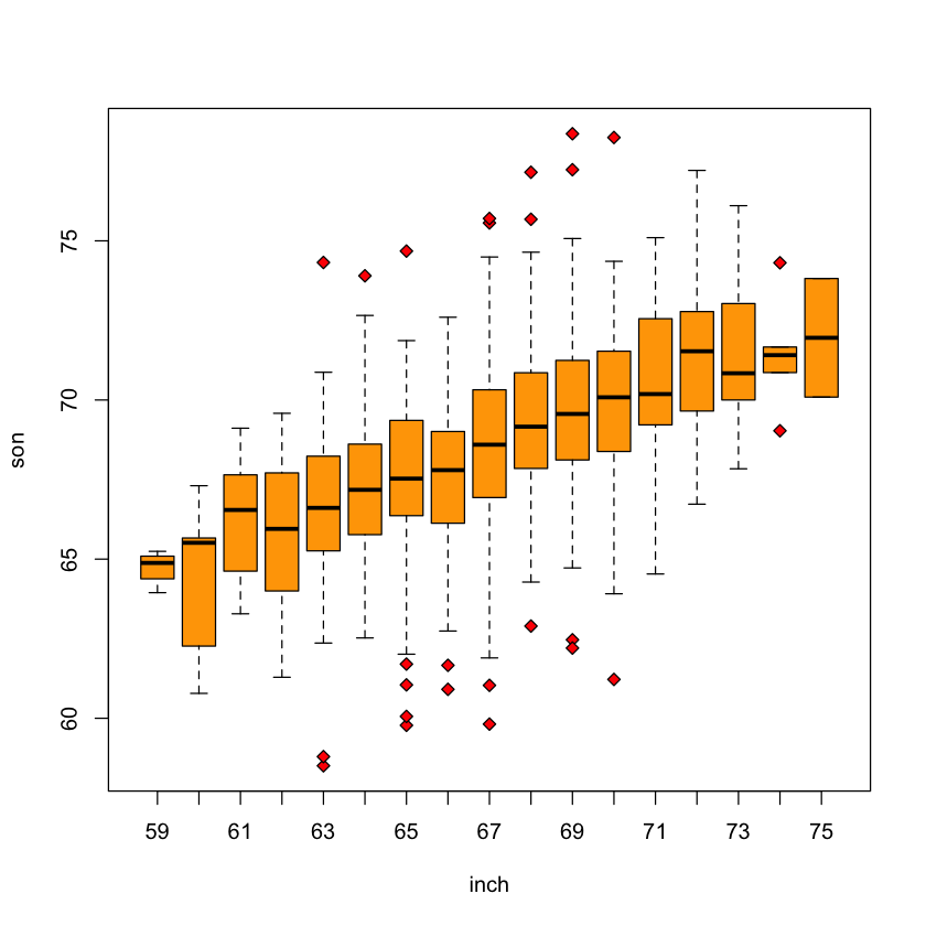
inch = factor(as.integer(father))
boxplot(son ~ inch,
        col='orange',
        pch=23,
        bg='red')

---

heights_fig + geom_abline(slope=slope, intercept=intercept, color='red', linewidth=3)

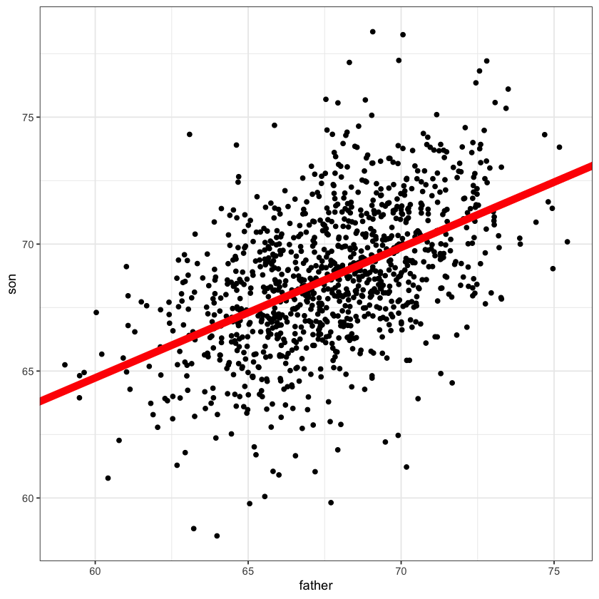
height.lm = lm(son ~ father, data=heights)
height.lm$coef

(Intercept)

33.8866043540779

father

0.514093038623309

---

What is a “regression” model?

• Model of the relationships between some covariates / predictors / features and an outcome.

• A regression model is a model of the average outcome given the covariates.

Mathematical formulation

For height data: a mathematical model:

\[ {\tt son} = f({\tt father}) + \varepsilon \]

• \(f\) describes how mean of son varies with father

• \(\varepsilon\) is the random variation within the slice.

---

{height=600 fig-align=”center”}

---

Linear regression models

• A linear regression model says that the function \(f\) is a sum (linear combination) of functions of father.

• Simple linear regression model:

(1)\[\begin{equation} f({\tt father}) = \beta_0 + \beta_1 \cdot {\tt father} \end{equation}\]

• Parameters of \(f\) are \((\beta_0, \beta_1)\)

• Could also be a sum (linear combination) of fixed functions of father:

(2)\[\begin{equation} f({\tt father}) = \beta_0 + \beta_1 \cdot {\tt father} + \beta_2 \cdot {\tt father}^2 \end{equation}\]

---

Statistical model

• Symbol \(Y\) usually used for outcomes, \(X\) for covariates…

• Model:

(3)\[\begin{equation} Y_i = \underbrace{\beta_0 + \beta_1 X_i}_{\text{regression equation}} + \underbrace{\varepsilon_i}_{\text{error}} \end{equation}\]

where \(\varepsilon_i \sim N(0, \sigma^2)\) are independent.

• This specifies a distribution for the \(Y\)’s given the \(X\)’s, i.e. it is a statistical model.

---

{height=600 fig-align=”center”}

Regression equation

• The regression equation is our slicewise model.

• Formally, this is a model of the conditional mean function

(4)\[\begin{equation} x \mapsto E[Y|X=x] \end{equation}\]

• Book uses the notation \(\mu\{Y|X\}\).

---

Fitting the model

• We will be using least squares regression. This measures the goodness of fit of a line by the sum of squared errors, \(SSE\).

• Least squares regression chooses the line that minimizes

(5)\[\begin{equation} SSE(\beta_0, \beta_1) = \sum_{i=1}^n (Y_i - \beta_0 - \beta_1 \cdot X_i)^2. \end{equation}\]

• In principle, we might measure goodness of fit differently:

  \[ SAD(\beta_0, \beta_1) = \sum_{i=1}^n |Y_i - \beta_0 - \beta_1 \cdot X_i|.\]

• For some other loss function \(L\) we might try to minimize

  \[ L(\beta_0,\beta_1) = \sum_{i=1}^n L(Y_i-\beta_0-\beta_1\cdot X_i) \]

---

Why least squares?

• With least squares, the minimizers have explicit formulae – not so important with today’s computer power.

• Resulting formulae are linear in the outcome \(Y\). This is important for inferential reasons. For only predictive power, this is also not so important.

• If assumptions are correct, then this is maximum likelihood estimation.

• Statistical theory tells us the maximum likelihood estimators (MLEs) are generally good estimators.

---

Choice of loss function

• Suppose we try to minimize squared error over \(\mu\):

\[ \sum_{i=1}^n (Y_i - \mu)^2. \]

• We know (by calculus) that the minimizer is the sample mean.

• If we minimize absolute error over \(\mu\)

\[ \sum_{i=1}^n |Y_i - \mu|.\]

• We know (similarly by calculus) that the minimizer(s) is (are) the sample median(s).

---

Visualizing the loss function

Let’s take some a random scatter plot and view the loss function.

X = rnorm(50)
Y = 1.5 + 0.1 * X + rnorm(50) * 2
parameters = lm(Y ~ X)$coef
intercept = parameters[1]
slope = parameters[2]
D = data.frame(X, Y)
ggplot(D, aes(X, Y)) + geom_point() + geom_abline(slope=slope, intercept=intercept)

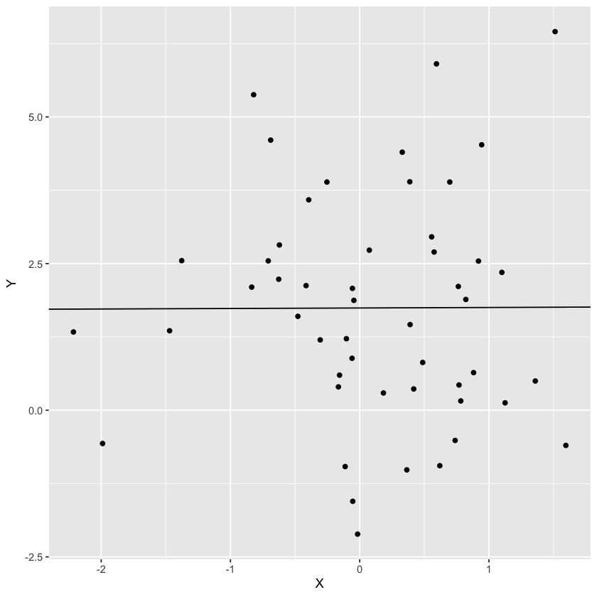
Let’s plot the loss as a function of the parameters. Note that the true intercept is 1.5 while the true slope is 0.1.

---

grid_intercept = seq(intercept - 2, intercept + 2, length=100)
grid_slope = seq(slope - 2, slope + 2, length=100)
loss_data = expand.grid(intercept=grid_intercept, slope=grid_slope)
loss_data$squared_error = numeric(nrow(loss_data))
for (i in 1:nrow(loss_data)) {
    loss_data$squared_error[i] = sum((D$Y - D$X * loss_data$slope[i] - loss_data$intercept[i])^2)
}
squared_error_fig = (ggplot(loss_data, aes(intercept, slope, fill=squared_error)) +
                     geom_raster() +
                     scale_fill_gradientn(colours=c("gray","yellow","blue")))
squared_error_fig

---

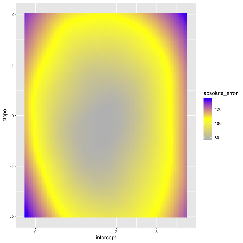
Let’s contrast this with the sum of absolute errors.

loss_data$absolute_error = numeric(nrow(loss_data))
for (i in 1:nrow(loss_data)) {
    loss_data$absolute_error[i] = sum(abs(D$Y - D$X * loss_data$slope[i] - loss_data$intercept[i]))
}
absolute_error_fig = (ggplot(loss_data, aes(intercept, slope, fill=absolute_error)) +
                      geom_raster() +
                      scale_fill_gradientn(colours=c("gray","yellow","blue")))
absolute_error_fig

---

Geometry of least squares

{height=600 fig-align=”center”}

• Some things to note:

  1. Minimizing sum of squares is the same as finding the point in the X,1 plane closest to \(Y\).

  2. The total dimension of the space is 1078.

  3. The dimension of the plane is 2-dimensional.

  4. The axis marked “\(\perp\)” should be thought of as \((n-2)\) dimensional, or, 1076 in this case.

---

Least squares

{height=600 fig-align=”center”}

The (squared) lengths of the above vectors are important quantities in what follows.

---

Important lengths

There are three to note:

(6)\[\begin{equation} \begin{aligned} SSE &= \sum_{i=1}^n(Y_i - \widehat{Y}_i)^2 = \sum_{i=1}^n (Y_i - \widehat{\beta}_0 - \widehat{\beta}_1 X_i)^2 \\ SSR &= \sum_{i=1}^n(\overline{Y} - \widehat{Y}_i)^2 = \sum_{i=1}^n (\overline{Y} - \widehat{\beta}_0 - \widehat{\beta}_1 X_i)^2 \\ SST &= \sum_{i=1}^n(Y_i - \overline{Y})^2 = SSE + SSR \\ \end{aligned} \end{equation}\]

---

An important summary of the fit is the ratio

(7)\[\begin{equation} \begin{aligned} R^2 &= \frac{SSR}{SST} \\ &= 1 - \frac{SSE}{SST} \\ &= \widehat{Cor}(\pmb{X},\pmb{Y})^2. \end{aligned} \end{equation}\]

• Measures how much variability in \(Y\) is explained by \(X\).

---

Case study A: data suggesting the Big Bang

url = 'https://raw.githubusercontent.com/StanfordStatistics/stats191-data/main/Sleuth3/big_bang.csv'
big_bang = read.table(url, sep=',', header=TRUE)
with(big_bang, plot(Velocity, Distance, pch=23, bg='red'))

---

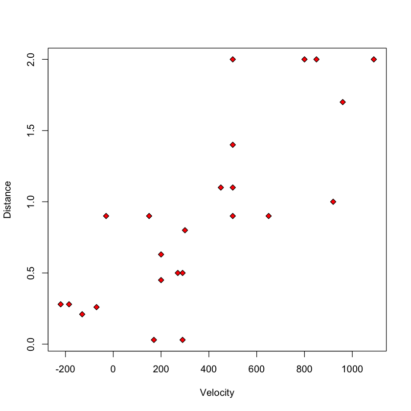
Let’s fit the linear regression model.

big_bang.lm = lm(Distance ~ Velocity, data=big_bang)
big_bang.lm

Call:
lm(formula = Distance ~ Velocity, data = big_bang)

Coefficients:
(Intercept)     Velocity  
   0.399170     0.001372  

---

Let’s look at the summary:

summary(big_bang.lm)

Call:
lm(formula = Distance ~ Velocity, data = big_bang)

Residuals:
     Min       1Q   Median       3Q      Max 
-0.76717 -0.23517 -0.01083  0.21081  0.91463 

Coefficients:
             Estimate Std. Error t value Pr(>|t|)    
(Intercept) 0.3991704  0.1186662   3.364   0.0028 ** 
Velocity    0.0013724  0.0002278   6.024 4.61e-06 ***
---
Signif. codes:  0 ‘***’ 0.001 ‘**’ 0.01 ‘*’ 0.05 ‘.’ 0.1 ‘ ’ 1

Residual standard error: 0.4056 on 22 degrees of freedom
Multiple R-squared:  0.6226,	Adjusted R-squared:  0.6054 
F-statistic: 36.29 on 1 and 22 DF,  p-value: 4.608e-06

---

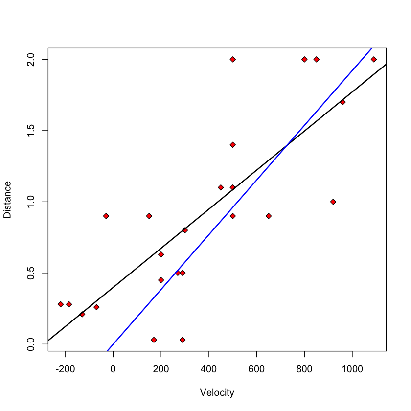
Hubble’s model

• Hubble’s theory of the Big Bang suggests that the correct slicewise (i.e. regression) model is

\[ \mu\{{\tt Distance} | {\tt Velocity}\} = \beta_1 \cdot {\tt Velocity} \]

• To fit without an intercept

hubble.lm = lm(Distance ~ Velocity - 1, data=big_bang)
summary(hubble.lm)

Call:
lm(formula = Distance ~ Velocity - 1, data = big_bang)

Residuals:
     Min       1Q   Median       3Q      Max 
-0.76767 -0.06909  0.22948  0.46056  1.03931 

Coefficients:
          Estimate Std. Error t value Pr(>|t|)    
Velocity 0.0019214  0.0001913   10.04 7.05e-10 ***
---
Signif. codes:  0 ‘***’ 0.001 ‘**’ 0.01 ‘*’ 0.05 ‘.’ 0.1 ‘ ’ 1

Residual standard error: 0.4882 on 23 degrees of freedom
Multiple R-squared:  0.8143,	Adjusted R-squared:  0.8062 
F-statistic: 100.9 on 1 and 23 DF,  p-value: 7.05e-10

---

with(big_bang, plot(Velocity, Distance, pch=23, bg='red'))
slope = coef(big_bang.lm)[1]
intercept = coef(big_bang.lm)[2]
abline(slope, intercept, lwd=2)
abline(0, coef(hubble.lm)[1], col='blue', lwd=2)

---

Least squares estimators

There are explicit formulae for the least squares estimators, i.e. the minimizers of the error sum of squares.

For the slope, \(\hat{\beta}_1\), it can be shown that

\[ \widehat{\beta}_1 = \frac{\sum_{i=1}^n(X_i - \overline{X})(Y_i - \overline{Y} )}{\sum_{i=1}^n (X_i-\overline{X})^2} = \frac{\widehat{Cov}(X,Y)}{\widehat{Var}( X)}.\]

Knowing the slope estimate, the intercept estimate can be found easily:

\[ \widehat{\beta}_0 = \overline{Y} - \widehat{\beta}_1 \cdot \overline{ X}.\]

---

Example: big_bang

beta.1.hat = with(big_bang, cov(Distance, Velocity) / var(Velocity))
beta.0.hat = with(big_bang, mean(Distance) - beta.1.hat * mean(Velocity))
c(beta.0.hat, beta.1.hat)
coef(big_bang.lm)

1. 0.399170439725205
2. 0.00137240753172474

(Intercept)

0.399170439725205

Velocity

0.00137240753172474

---

Estimate of \(\sigma^2\)

The estimate most commonly used is

\[\begin{split} \begin{aligned} \hat{\sigma}^2 &= \frac{1}{n-2} \sum_{i=1}^n (Y_i - \hat{\beta}_0 - \hat{\beta}_1 X_i)^2 \\ & = \frac{SSE}{n-2} \\ &= MSE \end{aligned} \end{split}\]

• We’ll use the common practice of replacing the quantity \(SSE(\hat{\beta}_0,\hat{\beta}_1)\), i.e. the minimum of this function, with just \(SSE\).

---

• The term MSE above refers to mean squared error: a sum of squares divided by its degrees of freedom. The degrees of freedom of SSE, the error sum of squares is therefore \(n-2\).

Mathematical aside

• We divide by \(n-2\) because some calculations tell us:

\[ \frac{\hat{\sigma}^2}{\sigma^2} \sim \frac{\chi^2_{n-2}}{n-2} \]

• Above, the right hand side denotes a chi-squared distribution with \(n-2\) degrees of freedom.

• Dividing by \(n-2\) gives an unbiased estimate of \(\sigma^2\) (assuming our modeling assumptions are correct).

---

Example: big_bang

sigma_hat = sqrt(sum(resid(big_bang.lm)^2) / big_bang.lm$df.resid)
sigma_hat
summary(big_bang.lm)

0.405630210825455

Call:
lm(formula = Distance ~ Velocity, data = big_bang)

Residuals:
     Min       1Q   Median       3Q      Max 
-0.76717 -0.23517 -0.01083  0.21081  0.91463 

Coefficients:
             Estimate Std. Error t value Pr(>|t|)    
(Intercept) 0.3991704  0.1186662   3.364   0.0028 ** 
Velocity    0.0013724  0.0002278   6.024 4.61e-06 ***
---
Signif. codes:  0 ‘***’ 0.001 ‘**’ 0.01 ‘*’ 0.05 ‘.’ 0.1 ‘ ’ 1

Residual standard error: 0.4056 on 22 degrees of freedom
Multiple R-squared:  0.6226,	Adjusted R-squared:  0.6054 
F-statistic: 36.29 on 1 and 22 DF,  p-value: 4.608e-06

---

Inference for the simple linear regression model

{height=400 fig-align=”center”}

Remember: \(X\) can be fixed or random in our model…

---

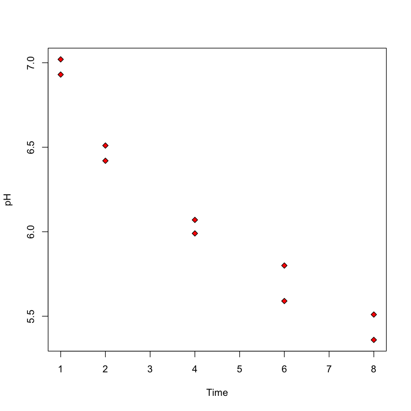
Case study B: predicting pH based on time after slaughter

• In this study, researches fixed \(X\) (Time) before measuring \(Y\) (pH)

• Ultimate goal: how long after slaughter is pH around 6?

url = 'https://raw.githubusercontent.com/StanfordStatistics/stats191-data/main/Sleuth3/meat_processing.csv'
meat_proc = read.table(url, sep=',', header=TRUE)
with(meat_proc, plot(Time, pH, pch=23, bg='red'))

---

Inference for \(\beta_0\) or \(\beta_1\)

• Recall our model

\[Y_i = \beta_0 + \beta_1 X_i + \varepsilon_i\]

• The errors \(\varepsilon_i\) are independent \(N(0, \sigma^2)\).

• In our heights example, we might want to now if there really is a linear association between \({\tt son}=Y\) and \({\tt father}=X\). This can be answered with a hypothesis test of the null hypothesis \(H_0:\beta_1=0\). This assumes the model above is correct, AND \(\beta_1=0\).

• Alternatively, we might want to have a range of values that we can be fairly certain \(\beta_1\) lies within. This is a confidence interval for \(\beta_1\).

---

A mathematical aside

• Let \(L\) be the subspace of \(\mathbb{R}^n\) spanned \(\pmb{1}=(1, \dots, 1)\) and \({X}=(X_1, \dots, X_n)\).

• We can decompose \(Y\) as

\[{Y} = P_L{Y} + ({Y} - P_L{Y}) = \widehat{{Y}} + (Y - \widehat{{Y}}) = \widehat{{Y}} + e\]

• In our model, \(\mu=\beta_0 \pmb{1} + \beta_1 {X} \in L\) so that

  \[ \widehat{{Y}} = \mu + P_L{\varepsilon}, \qquad {e} = P_{L^{\perp}}{{Y}} = P_{L^{\perp}}{\varepsilon}\]

• Our assumption that \(\varepsilon_i\)’s are independent \(N(0,\sigma^2)\) tells us that: \({e}\) and \(\widehat{{Y}}\) are independent; \(\widehat{\sigma}^2 = \|{e}\|^2 / (n-2) \sim \sigma^2 \cdot \chi^2_{n-2} / (n-2)\).

---

Setup for inference

• All of this implies

\[ \widehat{\beta}_1 \sim N\left(\beta_1, \frac{\sigma^2}{\sum_{i=1}^n(X_i-\overline{X})^2}\right).\]

• Therefore,

\[\frac{\widehat{\beta}_1 - \beta_1}{\sigma \cdot \sqrt{\frac{1}{\sum_{i=1}^n(X_i-\overline{X})^2}}} \sim N(0,1).\]

• The other quantity we need is the standard error or SE of \(\hat{\beta}_1\):

\[ SE(\widehat{\beta}_1) = \widehat{\sigma} \cdot \sqrt{\frac{1}{\sum_{i=1}^n(X_i-\overline{X})^2}} \qquad \text{independent of $\widehat{\beta}_1$}\]

---

Testing \(H_0:\beta_1=\beta_1^0\)

• Suppose we want to test that \(\beta_1\) is some pre-specified value, \(\beta_1^0\) (this is often 0: i.e. is there a linear association)

• Under \(H_0:\beta_1=\beta_1^0\)

  \[\frac{\widehat{\beta}_1 - \beta^0_1}{\widehat{\sigma} \sqrt{\frac{1}{\sum_{i=1}^n(X_i-\overline{X})^2}}} = \frac{\widehat{\beta}_1 - \beta^0_1}{ \frac{\widehat{\sigma}}{\sigma}\cdot \sigma \sqrt{\frac{1}{ \sum_{i=1}^n(X_i-\overline{X})^2}}} \sim t_{n-2}.\]

• Reject \(H_0:\beta_1=\beta_1^0\) if \(|T| > t_{n-2, 1-\alpha/2}\).

---

Example: big_bang

Let’s perform this test for the Big Bang data.

SE.beta.1.hat = with(big_bang, sigma_hat * sqrt(1 / sum((Velocity - mean(Velocity))^2)))
Tstat = (beta.1.hat - 0) / SE.beta.1.hat
c(estimate=beta.1.hat, SE=SE.beta.1.hat, T=Tstat)
summary(big_bang.lm)

estimate

0.00137240753172474

SE

0.00022782136747332

T

6.0240509788243

Call:
lm(formula = Distance ~ Velocity, data = big_bang)

Residuals:
     Min       1Q   Median       3Q      Max 
-0.76717 -0.23517 -0.01083  0.21081  0.91463 

Coefficients:
             Estimate Std. Error t value Pr(>|t|)    
(Intercept) 0.3991704  0.1186662   3.364   0.0028 ** 
Velocity    0.0013724  0.0002278   6.024 4.61e-06 ***
---
Signif. codes:  0 ‘***’ 0.001 ‘**’ 0.01 ‘*’ 0.05 ‘.’ 0.1 ‘ ’ 1

Residual standard error: 0.4056 on 22 degrees of freedom
Multiple R-squared:  0.6226,	Adjusted R-squared:  0.6054 
F-statistic: 36.29 on 1 and 22 DF,  p-value: 4.608e-06

---

• We see that R performs our \(t\)-test in the second row of the Coefficients table.

• It is clear that Distance is correlated with Velocity.

• There seems to be some flaw in Hubble’s theory: we reject \(H_0:\beta_0=0\) at level 5%: \(p\)-value is 0.0028!

---

Why reject for large |T|?

• Logic is the same as other \(t\) tests: observing a large \(|T|\) is unlikely if \(\beta_1 = \beta_1^0\) (i.e. if \(H_0\) were true). \(\implies\) it is reasonable to conclude that \(H_0\) is false.

• Common to report \(p\)-value:

\[\mathbb{P}(|T_{n-2}| > |T|_{obs}) = 2 \cdot \mathbb{P} (T_{n-2} > |T_{obs}|)\]

2*(1 - pt(Tstat, big_bang.lm$df.resid))
summary(big_bang.lm)

4.60768128074385e-06

Call:
lm(formula = Distance ~ Velocity, data = big_bang)

Residuals:
     Min       1Q   Median       3Q      Max 
-0.76717 -0.23517 -0.01083  0.21081  0.91463 

Coefficients:
             Estimate Std. Error t value Pr(>|t|)    
(Intercept) 0.3991704  0.1186662   3.364   0.0028 ** 
Velocity    0.0013724  0.0002278   6.024 4.61e-06 ***
---
Signif. codes:  0 ‘***’ 0.001 ‘**’ 0.01 ‘*’ 0.05 ‘.’ 0.1 ‘ ’ 1

Residual standard error: 0.4056 on 22 degrees of freedom
Multiple R-squared:  0.6226,	Adjusted R-squared:  0.6054 
F-statistic: 36.29 on 1 and 22 DF,  p-value: 4.608e-06

---

Confidence interval for regression parameters

• Applying the above to the parameter \(\beta_1\) yields a confidence interval of the form

\[\hat{\beta}_1 \pm SE(\hat{\beta}_1) \cdot t_{n-2, 1-\alpha/2}.\]

• Earlier, we computed \(SE(\hat{\beta}_1)\) using this formula

  \[ SE(a_0 \cdot \hat{\beta}_0 + a_1 \cdot \hat{\beta}_1) = \hat{\sigma} \sqrt{\frac{a_0^2}{n} + \frac{(a_0\cdot \overline{X} - a_1)^2}{\sum_{i=1}^n \left(X_i-\overline{X}\right)^2}}\]

with \((a_0,a_1) = (0, 1)\).

---

We also need to find the quantity \(t_{n-2,1-\alpha/2}\). This is defined by

\[ \mathbb{P}(T_{n-2} \geq t_{n-2,1-\alpha/2}) = \alpha/2. \]

In R, this is computed by the function qt.

alpha = 0.05
n = nrow(big_bang)
qt(1-0.5*alpha, n-2)
qnorm(1 - 0.5*alpha)

2.07387306790403

1.95996398454005

---

L = beta.1.hat - qt(0.975, big_bang.lm$df.resid) * SE.beta.1.hat
U = beta.1.hat + qt(0.975, big_bang.lm$df.resid) * SE.beta.1.hat
c(lower=L, upper=U)

lower

0.000899934933428759

upper

0.00184488013002073

We will not need to use these explicit formulae all the time, as R has some built in functions to compute confidence intervals.

confint(big_bang.lm)
confint(big_bang.lm, level=0.9)

A matrix: 2 × 2 of type dbl

	2.5 %	97.5 %
(Intercept)	0.1530719058	0.64526897
Velocity	0.0008999349	0.00184488

A matrix: 2 × 2 of type dbl

	5 %	95 %
(Intercept)	0.1954035267	0.60293735
Velocity	0.0009812054	0.00176361

Predicting the mean

Once we have estimated a slope \((\hat{\beta}_1)\) and an intercept \((\hat{\beta}_0)\), we can predict the height of the son born to a father of any particular height by the plugging-in the height of the new father, \(F_{new}\) into our regression equation:

\[ E[{S}_{new}|F_{new}] = \mu\{S_{new}|F_{new}\} = {\beta}_0 +{\beta}_1 F_{new}. \]

• Confidence interval for the average height of sons born to a father of height \(F_{new}=70\) (or maybe \(65\)) inches:

\[ \hat{\beta}_0 + 70 \cdot \hat{\beta}_1 \pm SE(\hat{\beta}_0 + 70 \cdot \hat{\beta}_1) \cdot t_{n-2, 1-\alpha/2}. \]

predict(height.lm,
        list(father=c(70, 65)),
	interval='confidence',
	level=0.90)

A matrix: 2 × 3 of type dbl

	fit	lwr	upr
1	69.87312	69.71333	70.03291
2	67.30265	67.13165	67.47366

---

new_fig = heights_fig + geom_abline(slope=slope, intercept=intercept, color='red', linewidth=3)
rect = data.frame(xmin=64.5, xmax=65.5, ymin=-Inf, ymax=Inf)
new_fig = new_fig + geom_rect(data=rect, aes(xmin=xmin, xmax=xmax, ymin=ymin, ymax=ymax),
                        color="grey20",
                        alpha=0.5,
                        inherit.aes = FALSE)
rect = data.frame(xmin=69.5, xmax=70.5, ymin=-Inf, ymax=Inf)
new_fig = new_fig + geom_rect(data=rect, aes(xmin=xmin, xmax=xmax, ymin=ymin, ymax=ymax),
                        color="grey20",
                        alpha=0.5,
                        inherit.aes = FALSE)
new_fig

---

Computing \(SE(\hat{\beta}_0 + 70 \cdot \hat{\beta}_1)\)

• We use the previous formula

  \[ SE(a_0\cdot \hat{\beta}_0 + a_1\cdot\hat{\beta}_1) = \hat{\sigma} \sqrt{\frac{a_0^2}{n} + \frac{(a_0\cdot \overline{X} - a_1)^2}{\sum_{i=1}^n \left(X_i-\overline{X}\right)^2}}\]

  with \((a_0, a_1) = (1, 70)\).

• Plugging in

\[ SE(\hat{\beta}_0 + 70 \cdot \hat{\beta}_1) = \hat{\sigma} \sqrt{\frac{1}{n} + \frac{(\overline{X} - 70)^2}{\sum_{i=1}^n \left(X_i-\overline{X}\right)^2}} \]

• As \(n\) grows (taking a larger sample), \(SE(\hat{\beta}_0 + 70 \hat{\beta}_1)\) should shrink to 0. Why?

---

Forecasting / prediction intervals

• Can we find an interval that covers the height of a particular son knowing only that her father’s height as 70 inches?

• Must cover the variability of the new random variation \(\implies\) it must be at least as wide as \(\sigma\).

---

#| fig-align: center
rect = data.frame(xmin=69.5, xmax=70.5, ymin=-Inf, ymax=Inf)
heights_fig + geom_rect(data=rect, aes(xmin=xmin, xmax=xmax, ymin=ymin, ymax=ymax),
                        color="grey20",
                        alpha=0.5,
                        inherit.aes = FALSE)

---

selected_points = (father <= 70.5) & (father >= 69.5)
center_ = mean(son[selected_points])
sd_ = sd(son[selected_points])
L = center_ - qnorm(0.95) * sd_
U = center_ + qnorm(0.95) * sd_
c(estimate=center_, lower=L, upper=U)

estimate

69.7684482608696

lower

65.6735353469882

upper

73.8633611747509

With so much data in our heights example, this 90% interval will have width roughly \(2 \cdot 1.96 \cdot \hat{\sigma}\)

sigma_hat_height = sqrt(sum(resid(height.lm)^2) / height.lm$df.resid)
c(2 * qnorm(0.95) * sigma_hat_height, U-L)

1. 8.01555526222726
2. 8.18982582776275

---

Formula

• Actual width will depend on how accurately we have estimated \((\beta_0, \beta_1)\) as well as \(\hat{\sigma}\).

\[ SE(\widehat{\beta}_0 + \widehat{\beta}_1 \cdot 70 + \varepsilon_{\text{new}}) = \widehat{\sigma} \sqrt{1 + \frac{1}{n} + \frac{(\overline{X} - 70)^2}{\sum_{i=1}^n \left(X_i-\overline{X}\right)^2}}. \]

The final interval is

\[ \hat{\beta}_0 + \hat{\beta}_1 \cdot 70 \pm t_{n-2, 1-\alpha/2} \cdot SE(\hat{\beta}_0 + \hat{\beta}_1 \cdot 70 + \varepsilon_{\text{new}}). \]

• Computed in R as follows

predict(height.lm, list(father=70), interval='prediction', level=0.90)

A matrix: 1 × 3 of type dbl

	fit	lwr	upr
1	69.87312	65.8587	73.88753