Multiple samples#
Download#
Outline#
Case studies:
Does diet affect longevity?
the Spock consipracy trial
Sums of squares
F-tests
set.seed(0)
Case study A: does diet affect longevity?#
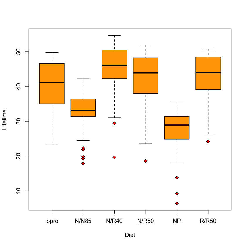
longevity = read.csv('https://raw.githubusercontent.com/StanfordStatistics/stats191-data/main/Sleuth3/longevity.csv', header=TRUE)
boxplot(Lifetime ~ Diet,
        data=longevity,
        col='orange',
        pch=23,
        bg='red')
One-way ANOVA model: generalization of two-sample#
 {height=400 fig-align=”center”}
Model details#
Data: \(Y_{ij}, 1 \leq i \leq n_j, j \in {\tt [lopro, N/N85, N/R40, N/R50, NP, R/R50]}\)
Model: \(Y_{ij} \sim N(\mu_j, \sigma^2)\) (Note: assumed equal variance here!)
Null: \(H_0\) no difference: \(\mu_{\tt lopro}=\dots=\mu_{\tt R/R50}\)
Alternative: \(H_a\) model holds for some values \(\mu_{\tt lopro},\dots,\mu_{\tt R/R50}\) but they are not all identical.
Fitting the model#
model = lm(Lifetime ~ Diet, data=longevity)
summary(model)
Call:
lm(formula = Lifetime ~ Diet, data = longevity)

Residuals:
     Min       1Q   Median       3Q      Max
-25.5167  -3.3857   0.8143   5.1833  10.0143

Coefficients:
            Estimate Std. Error t value Pr(>|t|)
(Intercept)  39.6857     0.8924  44.470  < 2e-16 ***
DietN/N85    -6.9945     1.2565  -5.567 5.25e-08 ***
DietN/R40     5.4310     1.2409   4.377 1.60e-05 ***
DietN/R50     2.6115     1.1936   2.188   0.0293 *
DietNP      -12.2837     1.3064  -9.403  < 2e-16 ***
DietR/R50     3.2000     1.2621   2.536   0.0117 *
---
Signif. codes:  0 ‘***’ 0.001 ‘**’ 0.01 ‘*’ 0.05 ‘.’ 0.1 ‘ ’ 1

Residual standard error: 6.678 on 343 degrees of freedom
Multiple R-squared:  0.4543,	Adjusted R-squared:  0.4463
F-statistic:  57.1 on 5 and 343 DF,  p-value: < 2.2e-16
Null model#
null_model = lm(Lifetime ~ 1, data=longevity)
summary(null_model)
Call:
lm(formula = Lifetime ~ 1, data = longevity)

Residuals:
    Min      1Q  Median      3Q     Max
-32.397  -6.997   0.703   8.103  15.803

Coefficients:
            Estimate Std. Error t value Pr(>|t|)
(Intercept)  38.7971     0.4804   80.76   <2e-16 ***
---
Signif. codes:  0 ‘***’ 0.001 ‘**’ 0.01 ‘*’ 0.05 ‘.’ 0.1 ‘ ’ 1

Residual standard error: 8.975 on 348 degrees of freedom
Comparing the models#
How much better a fit is model then null_model?#
Extra sum of squares#
SSE_F = sum(resid(model)^2)
SSE_R = sum(resid(null_model)^2)
SSE_R-SSE_F
12733.9418119068
\[\begin{split}
\begin{aligned}
SSE_R-SSE_F &= \|\hat{Y}_F-\hat{Y}_R\|^2_2 \\
&= \sum_{j=1}^6 \sum_{i=1}^{n_j}(\bar{Y}_j-\bar{Y}_{\cdot})^2
\end{aligned}
\end{split}\]
\(F\)-statistic#
Convert “extra” sum of squares to unitless quantity#
dfP = nrow(longevity) - 6
sdP = sqrt(sum(resid(model)^2) / dfP)
F = ((SSE_R-SSE_F) / 5) / sdP^2
F
57.1043140207422
\[
S^2_P = \frac{\sum_{j=1}^6 (n_j-1) \cdot S^2_j}{\sum_{j=1}^6 (n_j-1)}
\]
Using anova#
anova(null_model, model)
c(SSE_F, nrow(longevity)-6)
| Res.Df | RSS | Df | Sum of Sq | F | Pr(>F) | |
|---|---|---|---|---|---|---|
| <dbl> | <dbl> | <dbl> | <dbl> | <dbl> | <dbl> | |
| 1 | 348 | 28031.36 | NA | NA | NA | NA |
| 2 | 343 | 15297.42 | 5 | 12733.94 | 57.10431 | 4.111744e-43 |
- 15297.4153227636
- 343
Comparing two groups: N/N85 vs N/R50#
diff = with(longevity, mean(Lifetime[Diet=='N/N85']) - mean(Lifetime[Diet=='N/R50']))
sd_diff = with(longevity, sdP * sqrt(1/sum(Diet=='N/N85')+1/sum(Diet=='N/R50')))
T = (diff - 0) / sd_diff
T
-8.08798240038647
Confidence interval#
q = qt(0.975, 343)
c(L=diff-q*sd_diff, U=diff+q*sd_diff)
- L
- -11.9420127913839
- U
- -7.26989726544829
Comparing two groups: R/R50 vs N/R50#
diff = with(longevity, mean(Lifetime[Diet=='R/R50']) - mean(Lifetime[Diet=='N/R50']))
sd_diff = with(longevity, sdP * sqrt(1/sum(Diet=='N/N85')+1/sum(Diet=='N/R50')))
T = (diff - 0) / sd_diff
T
0.495529061862794
Confidence interval#
c(L=diff-q*sd_diff, U=diff+q*sd_diff)
- L
- -1.74752657584509
- U
- 2.92458895009056
Case study B: is the jury pool representative?#
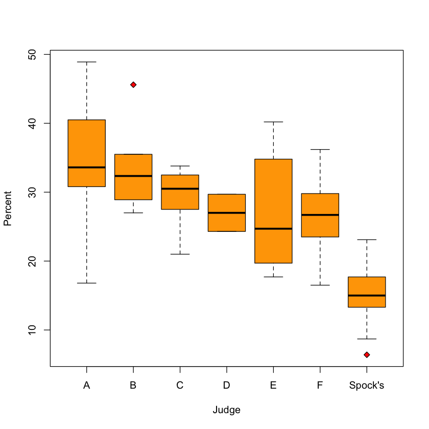
spock = read.csv('https://raw.githubusercontent.com/StanfordStatistics/stats191-data/main/Sleuth3/spock.csv', header=TRUE)
boxplot(Percent ~ Judge,
        data=spock,
        col='orange',
        pch=23,
        bg='red')
Any differences between judges?#
model_perc = lm(Percent ~ Judge, data=spock)
model0_perc = lm(Percent ~ 1, data=spock)
anova(model0_perc, model_perc)
| Res.Df | RSS | Df | Sum of Sq | F | Pr(>F) | |
|---|---|---|---|---|---|---|
| <dbl> | <dbl> | <dbl> | <dbl> | <dbl> | <dbl> | |
| 1 | 45 | 3791.526 | NA | NA | NA | NA |
| 2 | 39 | 1864.445 | 6 | 1927.081 | 6.718366 | 6.095823e-05 |
How about Spock’s judge vs. others?#
spock$Spock = spock$Judge == "Spock's"
modelS_perc = lm(Percent ~ Spock, data=spock)
summary(modelS_perc)
Call:
lm(formula = Percent ~ Spock, data = spock)

Residuals:
     Min       1Q   Median       3Q      Max
-12.9919  -4.6669   0.2581   3.7854  19.4081

Coefficients:
            Estimate Std. Error t value Pr(>|t|)
(Intercept)   29.492      1.160   25.42  < 2e-16 ***
SpockTRUE    -14.870      2.623   -5.67 1.03e-06 ***
---
Signif. codes:  0 ‘***’ 0.001 ‘**’ 0.01 ‘*’ 0.05 ‘.’ 0.1 ‘ ’ 1

Residual standard error: 7.056 on 44 degrees of freedom
Multiple R-squared:  0.4222,	Adjusted R-squared:  0.409
F-statistic: 32.15 on 1 and 44 DF,  p-value: 1.03e-06
Using anova#
anova(model0_perc, modelS_perc)
| Res.Df | RSS | Df | Sum of Sq | F | Pr(>F) | |
|---|---|---|---|---|---|---|
| <dbl> | <dbl> | <dbl> | <dbl> | <dbl> | <dbl> | |
| 1 | 45 | 3791.526 | NA | NA | NA | NA |
| 2 | 44 | 2190.903 | 1 | 1600.623 | 32.14538 | 1.029666e-06 |
How about variation only among others?#
anova(modelS_perc, model_perc)
| Res.Df | RSS | Df | Sum of Sq | F | Pr(>F) | |
|---|---|---|---|---|---|---|
| <dbl> | <dbl> | <dbl> | <dbl> | <dbl> | <dbl> | |
| 1 | 44 | 2190.903 | NA | NA | NA | NA |
| 2 | 39 | 1864.445 | 5 | 326.4579 | 1.365753 | 0.2581794 |
Summarizing all 3 models#
anova(model0_perc,
      modelS_perc,
      model_perc)
| Res.Df | RSS | Df | Sum of Sq | F | Pr(>F) | |
|---|---|---|---|---|---|---|
| <dbl> | <dbl> | <dbl> | <dbl> | <dbl> | <dbl> | |
| 1 | 45 | 3791.526 | NA | NA | NA | NA |
| 2 | 44 | 2190.903 | 1 | 1600.6230 | 33.481432 | 1.025824e-06 |
| 3 | 39 | 1864.445 | 5 | 326.4579 | 1.365753 | 2.581794e-01 |
Some diagnostic plots#
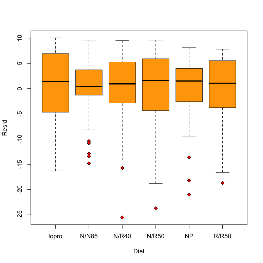
longevity study#
longevity$Resid = resid(model)
boxplot(Resid ~ Diet,
        data=longevity,
        col='orange',
        pch=23,
        bg='red')
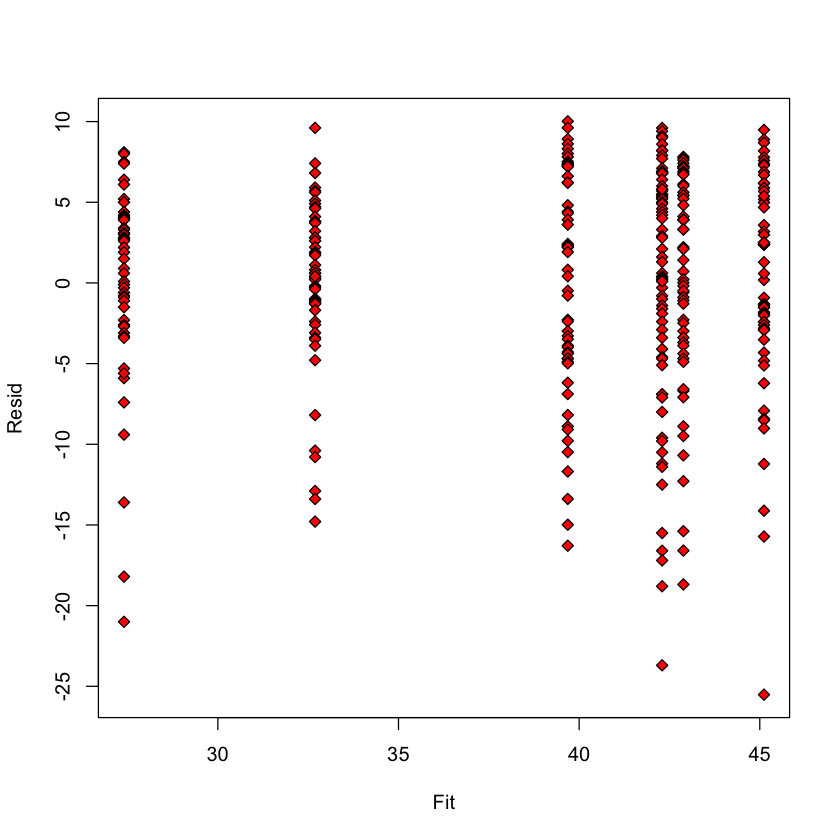
Residual vs. fitted#
longevity$Resid = resid(model)
longevity$Fit = predict(model)
with(longevity,
     plot(Fit, Resid,
          pch=23,
          bg='red'))
