Diagnostics I

Download

• Slides

• RStudio: RMarkdown,Quarto

• Jupyter

Ames Housing Data Set {.scrollable}

Here is a data set of house sales in Ames, IA.

df.housing <- read.csv("https://dlsun.github.io/data/housing.csv")
head(df.housing)

A data.frame: 6 × 6

	SaleMonth	SaleYear	SalePrice	Sqft	Bed	Bath
	<int>	<int>	<int>	<int>	<int>	<dbl>
1	1	2006	250000	2064	4	2.5
2	1	2006	401179	2795	4	3.5
3	1	2006	145000	1056	3	1.0
4	1	2006	181000	1309	3	1.5
5	1	2006	172400	1664	3	2.5
6	1	2006	252000	1964	3	2.5

…

Let’s use this data to build models to predict house prices!

Simple Linear Regression 1 {.scrollable}

How well does square footage predict house price?

…

with(df.housing, plot(Sqft, SalePrice))
simple.model.1 <- lm(SalePrice ~ Sqft, data=df.housing)
simple.model.1
abline(simple.model.1)

Call:
lm(formula = SalePrice ~ Sqft, data = df.housing)

Coefficients:
(Intercept)         Sqft  
    13289.6        111.7  

Simple Linear Regression 2 {.scrollable}

How well does number of bedrooms predict house price?

…

with(df.housing, plot(Bed, SalePrice))
simple.model.2 <- lm(SalePrice ~ Bed, data=df.housing)
simple.model.2
abline(simple.model.2)

Call:
lm(formula = SalePrice ~ Bed, data = df.housing)

Coefficients:
(Intercept)          Bed  
     141152        13889  

Simple Linear Regression 3 {.scrollable}

How well does number of bathrooms predict house price?

…

with(df.housing, plot(Bath, SalePrice))
simple.model.2 <- lm(SalePrice ~ Bath, data=df.housing)
simple.model.2
abline(simple.model.2)

Call:
lm(formula = SalePrice ~ Bath, data = df.housing)

Coefficients:
(Intercept)         Bath  
      54055        72163  

Multiple Linear Regression {.scrollable .smaller}

Let’s build a model that incorporates all of the predictors!

multiple.model <- lm(SalePrice ~ Sqft + Bed + Bath, data=df.housing)
multiple.model

Call:
lm(formula = SalePrice ~ Sqft + Bed + Bath, data = df.housing)

Coefficients:
(Intercept)         Sqft          Bed         Bath  
    51946.8        116.7     -30054.5      22529.8  

…

Why is the coefficient of Bed negative?

::: {.incremental}

• For each additional bedroom, the price of a home decreases by $30,054 on average, holding square footage constant. (Economists call this “ceteris paribus.”)

• If we increase the number of bedrooms without changing the square footage or the number of bathrooms, then each bedroom will be smaller, decreasing the house price. :::

Inference for Multiple Regression

What can we learn from inferential statistics?

summary(multiple.model)
confint(multiple.model)

Call:
lm(formula = SalePrice ~ Sqft + Bed + Bath, data = df.housing)

Residuals:
    Min      1Q  Median      3Q     Max 
-516716  -28082   -1978   24883  330612 

Coefficients:
              Estimate Std. Error t value Pr(>|t|)    
(Intercept)  51946.789   3739.458   13.89   <2e-16 ***
Sqft           116.733      2.875   40.61   <2e-16 ***
Bed         -30054.520   1349.251  -22.27   <2e-16 ***
Bath         22529.794   2117.394   10.64   <2e-16 ***
---
Signif. codes:  0 ‘***’ 0.001 ‘**’ 0.01 ‘*’ 0.05 ‘.’ 0.1 ‘ ’ 1

Residual standard error: 51640 on 2926 degrees of freedom
Multiple R-squared:  0.5825,	Adjusted R-squared:  0.5821 
F-statistic:  1361 on 3 and 2926 DF,  p-value: < 2.2e-16

A matrix: 4 × 2 of type dbl

	2.5 %	97.5 %
(Intercept)	44614.5535	59279.0238
Sqft	111.0963	122.3699
Bed	-32700.0984	-27408.9422
Bath	18378.0606	26681.5265

Assumptions of Linear Regression {.smaller .scrollable}

Inference for linear regression depends on the following assumptions:

::: {.incremental}

1. The linear model is correct: $\( \mu\{ Y | X_1, ..., X_p \} = \beta_0 + \beta_1 X_{1} + \dots + \beta_p X_{p}.\)\( In other words, \)\displaystyle Y_i = \beta_0 + \beta_1 X_{1i} + \dots + \beta_p X_{pi} + \text{error}_i.$

2. The errors are independent \(\text{Normal}(0, \sigma^2)\). :::

…

Assumption 2 is actually three assumptions in one:

::: {.incremental} a. The errors are normally distributed. b. The errors have constant variance. (Statisticians call this “homoskedasticity.”) c. The errors are independent. :::

…

How do we check these assumptions?

Residuals {.smaller}

::: {.incremental}

• We fit a linear regression model to the data and obtain $\( \hat\mu\{ Y | X_1, ..., X_p \} = \hat\beta_0 + \hat\beta_1 X_1 + \dots + \hat\beta_p X_p. \)$

• We can obtain the fitted values by plugging in the original data points: $\( \hat Y_i = \hat\beta_0 + \hat\beta_1 X_{i1} + \dots + \hat\beta_p X_{ip}. \)$

• The residuals are the difference between the actual values and the fitted values: $\( \begin{aligned} \text{residual}_i &= Y_i - \hat Y_i \\ &= (\beta_0 + \beta_1 X_{i1} + \dots + \beta_p X_{ip} + \text{error}_i) \\ &\quad - (\hat\beta_0 + \hat\beta_1 X_{i1} + \dots + \hat\beta_p X_{ip}) \\ &\approx \text{error}_i \end{aligned} \)$

• The residuals are an estimate of the errors! :::

Residual Plots {.scrollable}

To check assumptions about the errors, we can examine the residuals.

Example: To test the normality of the errors, make a normal Q-Q plot of the residuals.

qqnorm(multiple.model$resid)

Residual Plots {.scrollable}

To check assumptions about the errors, we can examine the residuals.

Example: To check correctness of the linear model and constant variance, plot the residuals against \(\hat Y\).

plot(multiple.model$fitted, multiple.model$resid)

Residual Plots {.scrollable}

If you call plot on a model fit using lm, then R will make many of these residual plots for you.

par(mfrow=c(2,2))
plot(multiple.model)

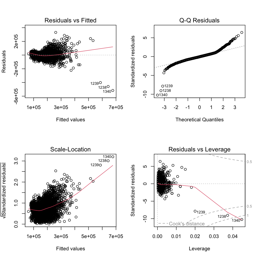
Conclusions

What have we learned from the residual analysis?

::: {.incremental}

• Linear model appears reasonable.

• Errors are not normal.

• Errors are not constant variance. :::

…

To fix these problems, we could consider transformations of \(Y\):

• log transformations: \(Y' = \ln(Y)\)

but we will not pursue that here.

Other Residual Plots

• Multiple regression models are fundamentally hard to visualize.

• Residuals can also help us visualize multiple regression models.

Partial Residual Plots {.smaller .scrollable}

A partial residual plot helps visualize the functional form of one predictor variable in a multiple regression model.

…

For example, the partial residuals of predictor \(X_k\) are defined by $\( \begin{aligned} \text{(partial residual for \)X_k\()}_i &= Y_i - \hat\beta_0 - \sum_{j\neq k} \hat\beta_j X_{ij} = \text{residual}_i + \hat\beta_k X_{ik} \end{aligned} \)$

…

A partial residual plot plots these partial residuals against \(X_k\).

partial.res <- multiple.model$resid + multiple.model$coef["Bed"] * df.housing$Bed
plot(df.housing$Bed, partial.res)

Partial Residual Models {.smaller .scrollable}

What if we fit a (simple) linear regression model to the partial residuals?

plot(df.housing$Bed, partial.res)
partial.res.model <- lm(partial.res ~ df.housing$Bed)
abline(partial.res.model)
summary(partial.res.model)

Call:
lm(formula = partial.res ~ df.housing$Bed)

Residuals:
    Min      1Q  Median      3Q     Max 
-516716  -28082   -1978   24883  330612 

Coefficients:
                 Estimate Std. Error t value Pr(>|t|)    
(Intercept)    -1.394e-09  3.425e+03    0.00        1    
df.housing$Bed -3.005e+04  1.152e+03  -26.08   <2e-16 ***
---
Signif. codes:  0 ‘***’ 0.001 ‘**’ 0.01 ‘*’ 0.05 ‘.’ 0.1 ‘ ’ 1

Residual standard error: 51620 on 2928 degrees of freedom
Multiple R-squared:  0.1885,	Adjusted R-squared:  0.1882 
F-statistic: 680.2 on 1 and 2928 DF,  p-value: < 2.2e-16

…

Where have we seen \(-30054\) before?

::: {.incremental}

• It is the coefficient of Bed in the multiple regression model!

• In general, the slope of the linear regression fit to the partial residuals will match the coefficient in the multiple regression.

• However, the standard error is not the same, so the inferences (\(p\)-value, confidence interval) will not match. :::

Partial Regression Plots {.smaller .scrollable}

A partial regression plot (also called an added variable plot) shows \(Y\) and \(X_k\), adjusting for the effect of the other predictors.

• residual of multiple regression of \(Y\) on \(X_1, \dots, X_{k-1}, X_{k+1}, \dots X_p\)

• residual of multiple regression of \(X_k\) on \(X_1, \dots, X_{k-1}, X_{k+1}, \dots X_p\)

…

res.y <- lm(SalePrice ~ Sqft + Bath, data=df.housing)$resid
res.x <- lm(Bed ~ Sqft + Bath, data=df.housing)$resid
plot(res.x, res.y)

Partial Regression Models {.smaller .scrollable}

A partial regression plot is harder to interpret than a partial residual plot (because both the \(x\) and \(y\) axes display residuals).

…

However, if we fit a (simple) linear regression model to the partial regression plot, the slope and inferences match the coefficient and inferences for Bed in the multiple regression exactly.

plot(res.x, res.y)
partial.reg.model <- lm(res.y ~ res.x)
abline(partial.reg.model)
summary(partial.reg.model)

Call:
lm(formula = res.y ~ res.x)

Residuals:
    Min      1Q  Median      3Q     Max 
-516716  -28082   -1978   24883  330612 

Coefficients:
              Estimate Std. Error t value Pr(>|t|)    
(Intercept) -2.320e-13  9.537e+02    0.00        1    
res.x       -3.005e+04  1.349e+03  -22.28   <2e-16 ***
---
Signif. codes:  0 ‘***’ 0.001 ‘**’ 0.01 ‘*’ 0.05 ‘.’ 0.1 ‘ ’ 1

Residual standard error: 51620 on 2928 degrees of freedom
Multiple R-squared:  0.145,	Adjusted R-squared:  0.1447 
F-statistic: 496.5 on 1 and 2928 DF,  p-value: < 2.2e-16