Assumptions for t tests

Download

• Slides

• RStudio: RMarkdown,Quarto

• Jupyter

Outline

• Case studies:

  1. Cloud seeding

  2. Effects of agent orange

• Robustness and resistance of two-sample \(t\)-tests

• Transformations

require(ggplot2)
set.seed(0)

Loading required package: ggplot2

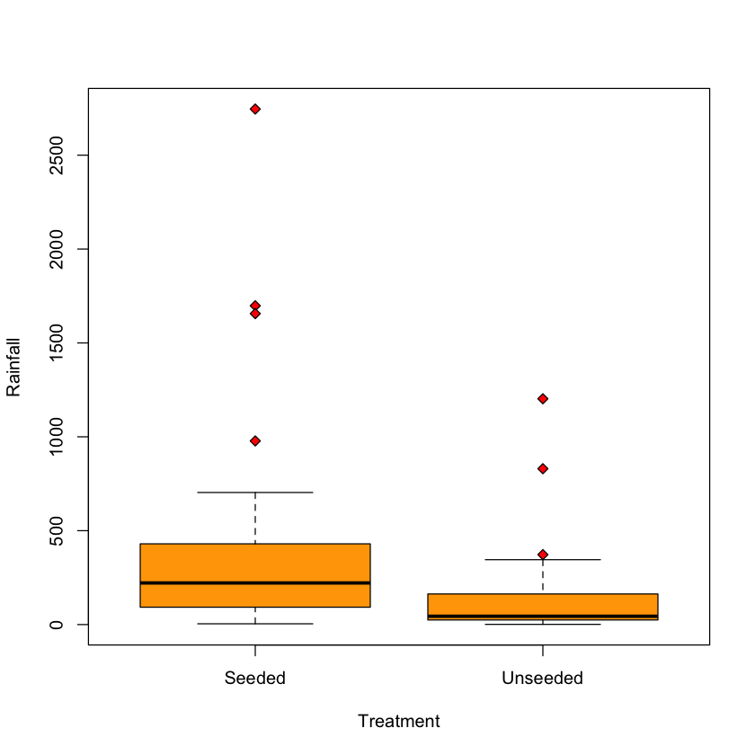
Case study A: effect of cloud seeding

rainfall = read.csv('https://raw.githubusercontent.com/StanfordStatistics/stats191-data/main/Sleuth3/rainfall.csv', header=TRUE)
boxplot(Rainfall ~ Treatment,
        data=rainfall,
        col='orange',
        pch=23,
        bg='red')

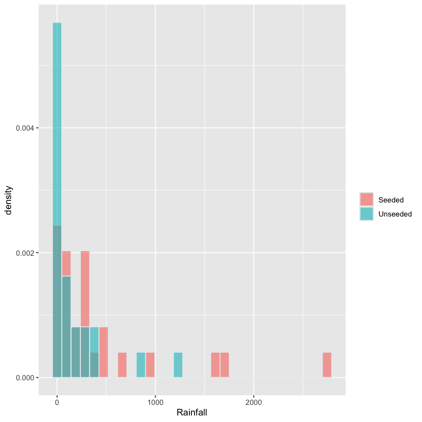
Histogram of Rainfall stratified by Treatment

# this plot is for visualization only
# students not expected to reproduce
rainfall = read.csv('https://raw.githubusercontent.com/StanfordStatistics/stats191-data/main/Sleuth3/rainfall.csv', header=TRUE)
fig <- (ggplot(rainfall, aes(x=Rainfall, fill=Treatment)) +
        geom_histogram(aes(y=after_stat(density)),
	               color="#e9ecef",
                       alpha=0.6,
                       position='identity',
		       bins=30) +
        labs(fill=""))
fig

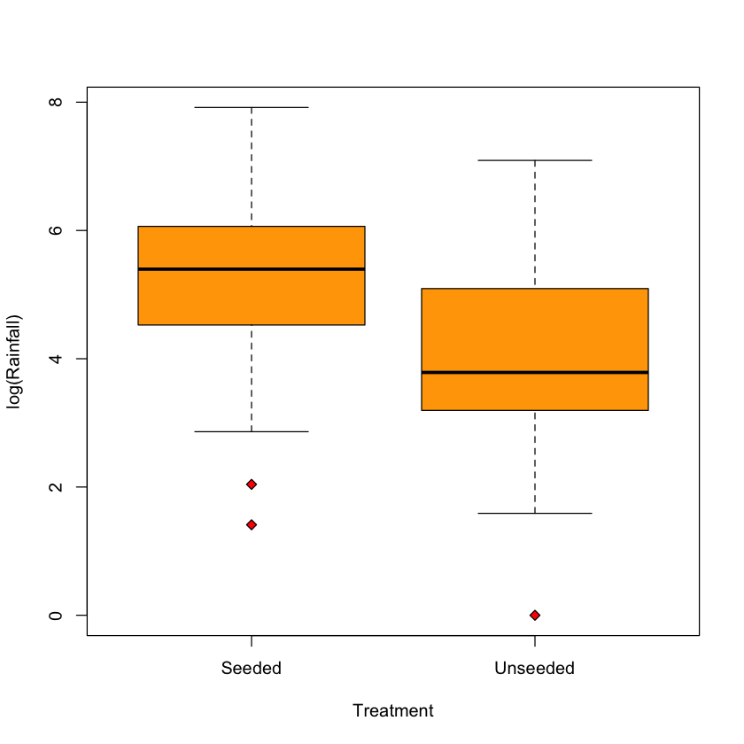
Practical tip: log transformation

boxplot(log(Rainfall) ~ Treatment,
        data=rainfall,
        col='orange',
        pch=23,
        bg='red')

Histogram of log(Rainfall) stratified by Treatment

# this plot is for visualization only
# students not expected to reproduce
rainfall$logRainfall = log(rainfall$Rainfall)
fig <- (ggplot(rainfall, aes(x=logRainfall, fill=Treatment)) +
        geom_histogram(aes(y=after_stat(density)),
                       color="#e9ecef",
                       alpha=0.6,
                       position='identity',
                       bins=30) +
        labs(fill=""))
fig

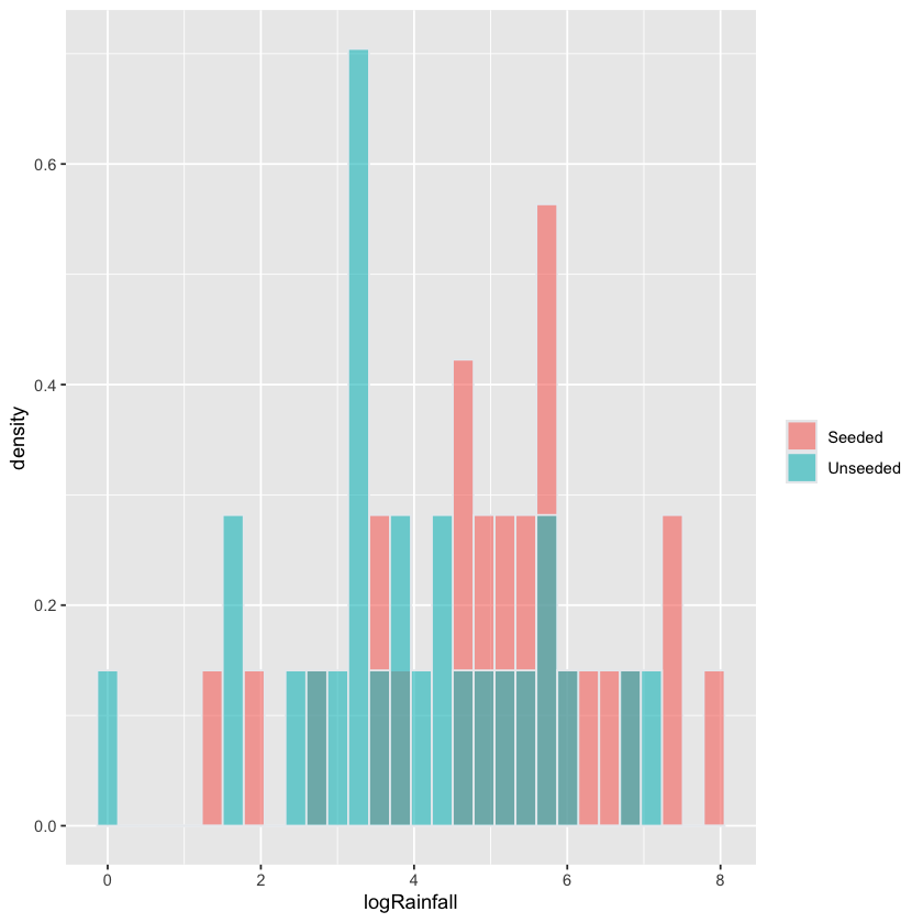
Does cloud seeding help?

• Histogram on log scale has similar shape for both groups \(\implies\) \(t\)-test probably well founded here.

t.test(log(Rainfall) ~ Treatment,
       var.equal=TRUE,
       data=rainfall)

	Two Sample t-test

data:  log(Rainfall) by Treatment
t = 2.5444, df = 50, p-value = 0.01408
alternative hypothesis: true difference in means between group Seeded and group Unseeded is not equal to 0
95 percent confidence interval:
 0.240865 2.046697
sample estimates:
  mean in group Seeded mean in group Unseeded 
              5.134187               3.990406 

Robustness of two sample \(t\)-tests

• Our analysis of beaks presumed \(\sigma^2_A=\sigma^2_B\) (as well as normality)

• What happens if:

  1. Unequal variance: \(\sigma^2_A \neq \sigma^2_B\)?

  2. Populations are not normal?

  3. Observations are not independent?

  4. Data are contaminated with outliers?

Mental model

{width=600 fig-align=”center”}

• Draw \(n_A\) samples from orange, \(n_B\) samples from purple.

Non-normality

Equal sample size \(n_A \approx n_B\)

• Some effect of long tails and skewness

Unequal sample size \(n_A \neq n_B\)

• Substantially affected by skewness

Skewness

• If skewness of distributions is quite different, \(t\) tools are affected for small and moderate sample sizes.

---

Unequal standard deviations \(\sigma^2_A \neq \sigma^2_B\)

• If \(n_A \approx n_B\) then small effect.

• Larger issue if \(n_A \neq n_B\).

Observations not being independent

• \(t\)-tests work poorly here

• Main problem is that \(SE\) will be off, usually we underestimate it…

---

Outlier

• A point in the data that is far from the others.

• Could be an accident in dataset construction, or could be due to long tails…

• Try analyzing data with / without candidate outliers

---

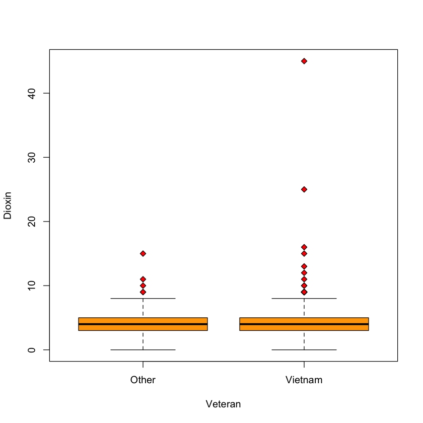
Case study B: dioxin in veterans

agent_orange = read.csv('https://raw.githubusercontent.com/StanfordStatistics/stats191-data/main/Sleuth3/agent_orange.csv', header=TRUE)
boxplot(Dioxin ~ Veteran,
        data=agent_orange,
        col='orange',
        pch=23,
        bg='red')

Histogram of Dioxin stratified by Veteran

# this plot is for visualization only
# students not expected to reproduce
agent_orange = read.csv('https://raw.githubusercontent.com/StanfordStatistics/stats191-data/main/Sleuth3/agent_orange.csv', header=TRUE)
fig <- (ggplot(agent_orange, aes(x=Dioxin, fill=Veteran)) +
        geom_histogram(aes(y=after_stat(density)),
	               color="#e9ecef",
		       alpha=0.6,
                       position='identity',
		       bins=30) +
        labs(fill=""))
fig

---

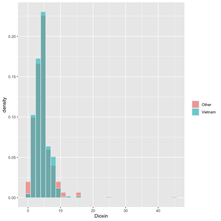
Outliers?

• Two Vietnam vets with level > 20

• Histograms have similar shape, so skewness similar + large sample sizes \(\implies\) \(t\)-test probably not too bad.

t.test(Dioxin ~ Veteran,
       var.equal=TRUE,
       data=agent_orange)

	Two Sample t-test

data:  Dioxin by Veteran
t = -0.26302, df = 741, p-value = 0.7926
alternative hypothesis: true difference in means between group Other and group Vietnam is not equal to 0
95 percent confidence interval:
 -0.6305128  0.4815229
sample estimates:
  mean in group Other mean in group Vietnam 
             4.185567              4.260062 

agent_orange$keep = agent_orange$Dioxin < 20
t.test(Dioxin ~ Veteran,
       var.equal=TRUE,
       subset=keep,
       data=agent_orange)$stat

t: 0.0969106642921687

Transformations

• We saw earlier that histogram for log(Rainfall) looked more “normal”.

• Using \(t\)-test on log(Rainfall) has \(\mu_{\tt Treated}\) as the mean of the log of rainfall after seeding…

Parameter \(\mu_{\tt Treated} - \mu_{\tt Untreated}\)

• Acts multiplicatively

Interpretation

• As noted in the book, the estimated effect is on log scale.

• Can be interpreted reasonably well when distribution of log-transformed data are symmetric.

• We estimate Treated has \(e^{5.13-3.99}\) multiplicative effect on median(Rainfall).