Logistic regression

Logistic regression#

Download#

Outline#

Case studies:

A. Survival in the Donner party

B. Smoking and bird-keeping
Binary outcomes
Estimation and inference: likelihood

Case study A: Donner party#

url = 'https://raw.githubusercontent.com/StanfordStatistics/stats191-data/main/Sleuth3/donner_party.csv'
donner.df = read.csv(url, sep=',', header=TRUE)
head(donner.df)

A data.frame: 6 × 3
	Age	Sex	Status
	<int>	<chr>	<chr>
1	23	Male	Died
2	40	Female	Survived
3	40	Male	Survived
4	30	Male	Died
5	28	Male	Died
6	40	Male	Died

Binary outcomes#

Most models so far have had response \(Y\) as continuous.
Status is Died/Survived
Other examples:
1. medical: presence or absence of cancer
2. financial: bankrupt or solvent
3. industrial: passes a quality control test or not

Modelling probabilities#

For \(0-1\) responses we need to model

\[\pi(x)=\pi(x_1, \dots, x_p) = P(Y=1|X_1=x_1,\dots, X_p=x_p)\]

That is, \(Y\) is Bernoulli with a probability that depends on covariates \(\{X_1, \dots, X_p\}.\)
Note: \(\text{Var}(Y|X) = \pi(X) ( 1 - \pi(X)) = E(Y|X) \cdot ( 1- E(Y|X))\)
Or, the binary nature forces a relation between mean and variance of \(Y\).
This makes logistic regression a Generalized Linear Model.

A possible model for `Donner`#

Set Y=Status=='Survived'
Simple model: lm(Y ~ Age + Sex)
Problems / issues:
1. We must have \(0 \leq E(Y|X) = \pi(X_1,X_2) \leq 1\). OLS will not force this.
2. Inference methods for will not work because of relation between mean and variance. Need to change how we compute variance!

Logistic regression#

Set X_1=Age, X_2=Sex
Logistic model

\[\pi(X_1,X_2) = \frac{\exp(\beta_0 + \beta_1 X_1 + \beta_2 X_2)}{1 + \exp(\beta_0 + \beta_1 X_1 + \beta_2 X_2)}\]

This automatically fixes \(0 \leq E(Y|X) = \pi(X_1,X_2) \leq 1\).

Logit transform#

Definition: \(\text{logit}(\pi(X_1, X_2)) = \log\left(\frac{\pi(X_1, X_2)}{1 - \pi(X_1,X_2)}\right) = \beta_0 + \beta_1 X_1 + \beta_2 X_2\)

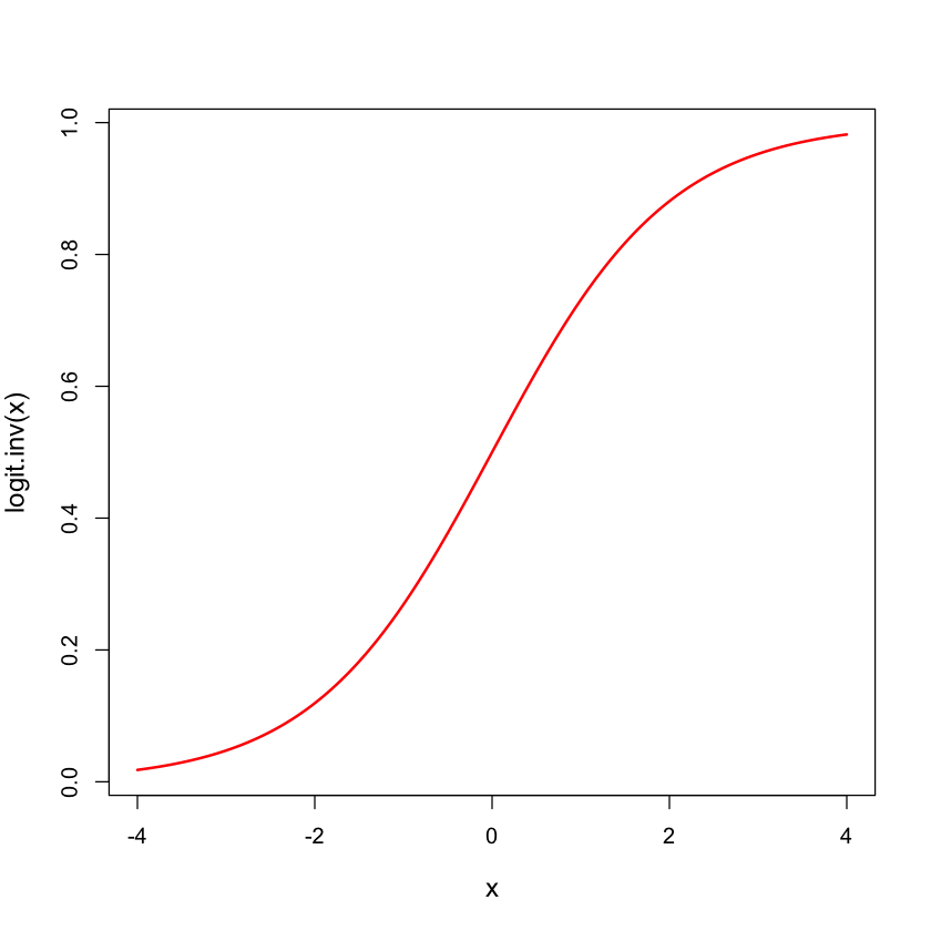
Logistic distribution#

logit.inv = function(x) {
  return(exp(x) / (1 + exp(x)))
}
x = seq(-4, 4, length=200)
plot(x, logit.inv(x), lwd=2, type='l', col='red', cex.lab=1.2)

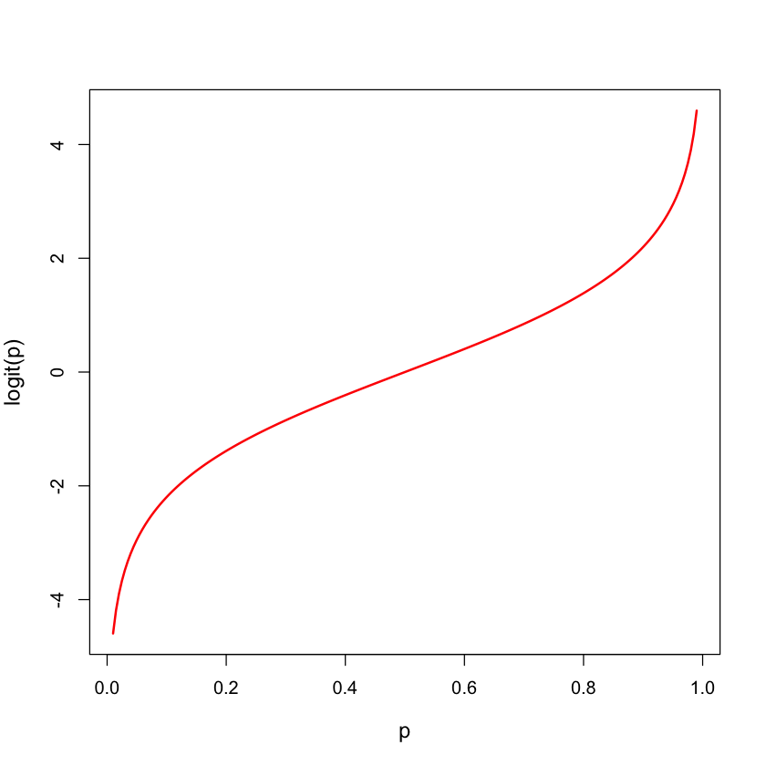
../../_images/9e3e290d3b6dfde3198138acc1ccef5b859e1f6e9ea8afa5fc3fa41450e3ebb7.png

Logistic transform: `logit`#

logit = function(p) {
  return(log(p / (1 - p)))
}
p = seq(0.01,0.99,length=200)
plot(p, logit(p), lwd=2, type='l', col='red', cex.lab=1.2)

../../_images/9745e8427e44bebf9d9523c9140558f175ab00578775b625e2ffc80c2c495d12.png

Binary regression models#

Models \(E(Y)\) as \(F(\beta_0 + \beta_1 X_1 + \beta_2 X_2)\) for some increasing function \(F\) (usually a distribution function).
The logistic model uses the function (we called logit.inv above)

\[F(x)=\frac{e^x}{1+e^x}.\]

Can be fit using Maximum Likelihood / Iteratively Reweighted Least Squares.
For logistic regression, coefficients have nice interpretation in terms of odds ratios (to be defined shortly).
What about inference?

Criterion used to fit model#

Instead of sum of squares, logistic regression uses deviance:

\(DEV(\mu| Y) = -2 \log L(\mu| Y) + 2 \log L(Y| Y)\) where \(\mu\) is a location estimator for \(Y\).
If \(Y\) is Gaussian with independent \(N(\mu_i,\sigma^2)\) entries then \(DEV(\mu| Y) = \frac{1}{\sigma^2}\sum_{i=1}^n(Y_i - \mu_i)^2\)
If \(Y\) is a binary vector, with mean vector \(\pi\) then \(DEV(\pi| Y) = -2 \sum_{i=1}^n \left( Y_i \log(\pi_i) + (1-Y_i) \log(1-\pi_i) \right)\)
Minimizing deviance \(\iff\) Maximum Likelihood

Deviance for logistic regression#

For any binary regression model, \(\pi=\pi(\beta)\).
The deviance is:

\[\begin{aligned} DEV(\beta| Y) &= -2 \sum_{i=1}^n \left( Y_i {\text{logit}}(\pi_i(\beta)) + \log(1-\pi_i(\beta)) \right) \end{aligned}\]

For the logistic model, the RHS is:

\[ \begin{aligned} -2 \left[ (X\beta)^Ty + \sum_{i=1}^n\log \left(1 + \exp \left(\beta_0 + \sum_{j=1}^p X_{ij} \beta_j\right) \right)\right] \end{aligned}\]

The logistic model is special in that \(\text{logit}(\pi(\beta))=X\beta\). If we used a different transformation, the first part would not be linear in \(X\beta\).

donner.df$Y = donner.df$Status == 'Survived'
donner.glm = glm(Y ~ Age + Sex, data=donner.df,
                 family=binomial())
summary(donner.glm)

Call:
glm(formula = Y ~ Age + Sex, family = binomial(), data = donner.df)

Coefficients:
            Estimate Std. Error z value Pr(>|z|)  
(Intercept)  3.23041    1.38686   2.329   0.0198 *
Age         -0.07820    0.03728  -2.097   0.0359 *
SexMale     -1.59729    0.75547  -2.114   0.0345 *
---
Signif. codes:  0 ‘***’ 0.001 ‘**’ 0.01 ‘*’ 0.05 ‘.’ 0.1 ‘ ’ 1

(Dispersion parameter for binomial family taken to be 1)

    Null deviance: 61.827  on 44  degrees of freedom
Residual deviance: 51.256  on 42  degrees of freedom
AIC: 57.256

Number of Fisher Scoring iterations: 4

Odds Ratios#

One reason logistic models are popular is that the parameters have simple interpretations in terms of odds

\[ODDS(A) = \frac{P(A)}{1-P(A)}.\]
Logistic model:

\[OR_{X_j} = \frac{ODDS(Y=1|\dots, X_j=x_j+h, \dots)}{ODDS(Y=1|\dots, X_j=x_j, \dots)} = e^{h \beta_j}\]

If \(X_j \in {0, 1}\) is dichotomous, then odds for group with \(X_j = 1\) are \(e^{\beta_j}\) higher, other parameters being equal.

Tempting to think of odds ratio as probability ratio, but not quite the same
In Donner, the odds ratio for a 45 year old male compared to a 35 year old female

\[e^{-0.7820-1.5973}=-2.3793\]

logodds = predict(donner.glm, list(Age=c(35,45),Sex=c('Female', 'Male')),
                 type='link')
logodds
logodds[2] - logodds[1]
exp(logodds[2] - logodds[1])

1: 0.493271271049863
2: -1.88606295597673

2: -2.37933422702659

2: 0.0926122156997664

The estimated probabilities yield a ratio of \(0.1317/0.6209 \approx 0.21\).

prob = exp(logodds)/(1+exp(logodds))
prob
prob[2] / prob[1]

1: 0.620876756856824
2: 0.131694020754108

2: 0.212109761397426

When success is rare (rare disease hypothesis) then odds ratios are approximately probability ratios…

Inference#

Model is fit to minimize deviance
Fit using IRLS (Iteratively Reweighted Least Squares) algorithm
General formula for \(\text{Var}(\hat{\beta})\) from IRLS.
Intervals formed width vcov() are called Wald intervals.

center = coef(donner.glm)['Age']
SE = sqrt(vcov(donner.glm)['Age', 'Age'])
U = center + SE * qnorm(0.975)
L = center - SE * qnorm(0.975)
data.frame(L, center, U)

A data.frame: 1 × 3
	L	center	U
	<dbl>	<dbl>	<dbl>
Age	-0.1512803	-0.07820407	-0.005127799

Covariance#

The estimated covariance uses the “weights” computed from the fitted model.

pi.hat = fitted(donner.glm)
W.hat = pi.hat * (1 - pi.hat)
X = model.matrix(donner.glm)
C = solve(t(X) %*% (W.hat * X))
c(SE, sqrt(C['Age', 'Age']))

0.0372844979677129
0.0372874889556373

Confidence intervals#

The intervals above are slightly different from what R will give you if you ask it for confidence intervals.
R uses so-called profile intervals.
For large samples the two methods should agree quite closely.

CI = confint(donner.glm)
CI
mean(CI[2,]) # profile intervals are not symmetric around the estimate...
data.frame(L, center, U)

Waiting for profiling to be done...

A matrix: 3 × 2 of type dbl
	2.5 %	97.5 %
(Intercept)	0.8514190	6.42669512
Age	-0.1624377	-0.01406576
SexMale	-3.2286705	-0.19510198

-0.0882517038296134

A data.frame: 1 × 3
	L	center	U
	<dbl>	<dbl>	<dbl>
Age	-0.1512803	-0.07820407	-0.005127799

Example from book#

The book considers testing whether there is any interaction between Sex and Age in the Donner party data:

summary(glm(Y ~ Age + Sex + Age:Sex, 
            donner.df, 
            family=binomial()))$coef

A matrix: 4 × 4 of type dbl
	Estimate	Std. Error	z value	Pr(>\|z\|)
(Intercept)	7.2463848	3.20516725	2.260845	0.02376889
Age	-0.1940741	0.08741539	-2.220137	0.02640948
SexMale	-6.9280495	3.39887166	-2.038338	0.04151614
Age:SexMale	0.1615969	0.09426191	1.714339	0.08646650

\(Z\)-test for testing \(H_0:\beta_{\texttt Age:SexMale}=0\):

\[ Z = \frac{0.1616-0}{0.09426} \approx 1.714 \]

When \(H_0\) is true, \(Z\) is approximately \(N(0,1)\).

pval = 2 * pnorm(1.714, lower=FALSE)
pval

0.0865287258673211

Comparing models in logistic regression#

For a model \({\cal M}\), \(DEV({\cal M})\) replaces \(SSE({\cal M})\).
In least squares regression (with \(\sigma^2\) known), we use

\[\frac{1}{\sigma^2}\left( SSE({\cal M}_R) - SSE({\cal M}_F) \right) \overset{H_0:{\cal M}_R}{\sim} \chi^2_{df_R-df_F}\]

This is closely related to \(F\) with large \(df_F\): approximately \(F_{df_R-df_F, df_F} \cdot (df_R-df_F)\).
For logistic regression this difference in \(SSE\) is replaced with

\[DEV({\cal M}_R) - DEV({\cal M}_F) \overset{n \rightarrow \infty, H_0:{\cal M}_R}{\sim} \chi^2_{df_R-df_F}\]

Resulting tests do not agree numerically with those coming from IRLS (Wald tests). Both are often used.

Comparing `~ Age + Sex` to `~1`#

anova(glm(Y ~ 1,
          data=donner.df, 
          family=binomial()), 
      donner.glm)

A anova: 2 × 5
	Resid. Df	Resid. Dev	Df	Deviance	Pr(>Chi)
	<dbl>	<dbl>	<dbl>	<dbl>	<dbl>
1	44	61.82654	NA	NA	NA
2	42	51.25628	2	10.57026	0.00506638

Corresponding \(p\)-value:

1 - pchisq(10.57, 2) # testing ~1 vs ~1 + Health.Aware + Age

0.00506703218816074

Comparing `~ Age + Sex` to `~ Age`#

anova(glm(Y ~ Age,
          data=donner.df, 
          family=binomial()), 
      donner.glm)

A anova: 2 × 5
	Resid. Df	Resid. Dev	Df	Deviance	Pr(>Chi)
	<dbl>	<dbl>	<dbl>	<dbl>	<dbl>
1	43	56.29072	NA	NA	NA
2	42	51.25628	1	5.034437	0.02484816

Corresponding \(p\)-value:

1 - pchisq(5.03, 1) # testing ~ 1 + Health.Aware vs ~1 + Health.Aware + Age

0.024911898430907

Let’s compare this with the Wald test:

summary(donner.glm)

Call:
glm(formula = Y ~ Age + Sex, family = binomial(), data = donner.df)

Coefficients:
            Estimate Std. Error z value Pr(>|z|)  
(Intercept)  3.23041    1.38686   2.329   0.0198 *
Age         -0.07820    0.03728  -2.097   0.0359 *
SexMale     -1.59729    0.75547  -2.114   0.0345 *
---
Signif. codes:  0 ‘***’ 0.001 ‘**’ 0.01 ‘*’ 0.05 ‘.’ 0.1 ‘ ’ 1

(Dispersion parameter for binomial family taken to be 1)

    Null deviance: 61.827  on 44  degrees of freedom
Residual deviance: 51.256  on 42  degrees of freedom
AIC: 57.256

Number of Fisher Scoring iterations: 4

Diagnostics#

Similar to least square regression, only residuals used are usually deviance residuals

\[r_i = \text{sign}(Y_i-\widehat{\pi}_i) \sqrt{DEV(\widehat{\pi}_i|Y_i)}.\]
These agree with usual residual for least square regression.

par(mfrow=c(2,2))
plot(donner.glm)

../../_images/132198aaf47d1cfadfae2d0a61aafbb3a441d4b114b3b5ebc785390780b1589c.png

influence.measures(donner.glm)

Influence measures of
	 glm(formula = Y ~ Age + Sex, family = binomial(), data = donner.df) :

    dfb.1_  dfb.Age dfb.SxMl   dffit cov.r   cook.d    hat inf
-0.0828  0.09169  -0.0900 -0.2341 1.047 0.015372 0.0492    
 0.0228  0.13667  -0.2285  0.3671 1.100 0.038310 0.1025    
-0.2909  0.32202   0.2497  0.4314 0.916 0.094717 0.0567    
 0.0308 -0.03411  -0.0974 -0.1648 1.065 0.006840 0.0387    
 0.0047 -0.00520  -0.0971 -0.1763 1.058 0.008042 0.0389    
 0.0972 -0.10766  -0.0835 -0.1442 1.111 0.004763 0.0567    
 0.0701 -0.23190   0.1880 -0.3990 1.146 0.043320 0.1310    
 0.0599 -0.06636  -0.0309 -0.0697 1.146 0.001030 0.0670    
 0.0518 -0.05738  -0.0259 -0.0598 1.143 0.000756 0.0628    
0.0701 -0.23190   0.1880 -0.3990 1.146 0.043320 0.1310    
-0.3939  0.23169   0.4066 -0.4886 0.955 0.109490 0.0780    
-0.0071  0.00786   0.1466  0.2663 0.986 0.024482 0.0389    
0.0047 -0.00520  -0.0971 -0.1763 1.058 0.008042 0.0389    
-0.0828  0.09169  -0.0900 -0.2341 1.047 0.015372 0.0492    
0.1534 -0.10271  -0.1414  0.1748 1.139 0.006983 0.0802    
0.1543 -0.09959  -0.1473  0.1801 1.136 0.007465 0.0794    
-0.0071  0.00786   0.1466  0.2663 0.986 0.024482 0.0389    
0.1342 -0.10552  -0.1022  0.1391 1.155 0.004259 0.0839    
0.1005 -0.25632   0.1656 -0.3986 1.172 0.041875 0.1438    
0.0744 -0.08240  -0.0408 -0.0880 1.150 0.001656 0.0721    
0.1500 -0.10660  -0.1298  0.1644 1.145 0.006103 0.0817    
0.1714 -0.18980   0.0614  0.2872 1.076 0.022793 0.0735    
-0.0439  0.04860  -0.0940 -0.2054 1.050 0.011427 0.0433    
0.0656 -0.07267  -0.0346 -0.0768 1.148 0.001254 0.0694    
0.0557 -0.06172   0.1193  0.2608 1.009 0.021757 0.0433    
0.1434 -0.15882   0.0768  0.2773 1.055 0.022058 0.0623    
-0.0992  0.10982   0.1833  0.2998 0.962 0.034818 0.0403    
0.1259 -0.02425  -0.1980  0.2436 1.109 0.014897 0.0786    
0.1546 -0.09559  -0.1532  0.1855 1.133 0.007983 0.0787    
-0.0522  0.05781   0.1650  0.2793 0.974 0.028470 0.0387    
-0.2884  0.31929  -0.0567 -0.4225 1.046 0.059528 0.0928    
0.1370 -0.28212   0.1339 -0.3937 1.211 0.039152 0.1626    
0.1520 -0.10503  -0.1355  0.1695 1.142 0.006530 0.0810    
-0.0439  0.04860  -0.0940 -0.2054 1.050 0.011427 0.0433    
-0.4172  0.46184   0.2851  0.5385 0.876 0.187509 0.0685    
0.1259 -0.02425  -0.1980  0.2436 1.109 0.014897 0.0786    
0.0308 -0.03411  -0.0974 -0.1648 1.065 0.006840 0.0387    
-0.0439  0.04860  -0.0940 -0.2054 1.050 0.011427 0.0433    
-0.0439  0.04860  -0.0940 -0.2054 1.050 0.011427 0.0433    
-0.0439  0.04860  -0.0940 -0.2054 1.050 0.011427 0.0433    
0.0308 -0.03411  -0.0974 -0.1648 1.065 0.006840 0.0387    
0.0761 -0.08422  -0.0931 -0.1518 1.087 0.005495 0.0453    
0.0937 -0.10368   0.1018  0.2648 1.026 0.021407 0.0492    
-0.0627  0.06942  -0.0922 -0.2188 1.049 0.013186 0.0459    
0.1541 -0.09064  -0.1591  0.1912 1.130 0.008544 0.0780    

Model selection#

Models all have AIC scores \(\implies\) stepwise selection can be used easily!
Package bestglm has something like leaps functionality (not covered here)

AIC(donner.glm)
null.glm = glm(Y ~ 1, data=donner.df, family=binomial())
upper.glm = glm(Y ~ (.-Status)^2, data=donner.df, family=binomial())
donner_selected = step(null.glm, scope=list(upper=upper.glm), direction='both')
summary(donner_selected)$coef

57.2562845365773

Start:  AIC=63.83
Y ~ 1

       Df Deviance    AIC
+ Age   1   56.291 60.291
+ Sex   1   57.286 61.286
<none>      61.827 63.827

Step:  AIC=60.29
Y ~ Age

       Df Deviance    AIC
+ Sex   1   51.256 57.256
<none>      56.291 60.291
- Age   1   61.827 63.827

Step:  AIC=57.26
Y ~ Age + Sex

          Df Deviance    AIC
+ Age:Sex  1   47.346 55.346
<none>         51.256 57.256
- Sex      1   56.291 60.291
- Age      1   57.286 61.286

Step:  AIC=55.35
Y ~ Age + Sex + Age:Sex

          Df Deviance    AIC
<none>         47.346 55.346
- Age:Sex  1   51.256 57.256

A matrix: 4 × 4 of type dbl
	Estimate	Std. Error	z value	Pr(>\|z\|)
(Intercept)	7.2463848	3.20516725	2.260845	0.02376889
Age	-0.1940741	0.08741539	-2.220137	0.02640948
SexMale	-6.9280495	3.39887166	-2.038338	0.04151614
Age:SexMale	0.1615969	0.09426191	1.714339	0.08646650

Case Study B: birdkeeping and smoking#

Outcome: LC, lung cancer status
Features:
1. FM: sex of patient
2. AG: age (years)
3. SS: socio-economic status
4. YR: years of smoking prior to examination / diagnosis
5. CD: cigarettes per day
6. BK: whether or not subjects keep birds at home

url = 'https://raw.githubusercontent.com/StanfordStatistics/stats191-data/main/Sleuth3/smoking_birds.csv'
smoking.df = read.csv(url, sep=',', header=TRUE)
smoking.df$LC = smoking.df$LC == 'LungCancer'
head(smoking.df)

A data.frame: 6 × 7
	LC	FM	SS	BK	AG	YR	CD
	<lgl>	<chr>	<chr>	<chr>	<int>	<int>	<int>
1	TRUE	Male	Low	Bird	37	19	12
2	TRUE	Male	Low	Bird	41	22	15
3	TRUE	Male	High	NoBird	43	19	15
4	TRUE	Male	Low	Bird	46	24	15
5	TRUE	Male	Low	Bird	49	31	20
6	TRUE	Male	High	NoBird	51	24	15

base.glm = glm(LC ~ .,
               data=smoking.df,
               family=binomial())
summary(base.glm)$coef

A matrix: 7 × 4 of type dbl
	Estimate	Std. Error	z value	Pr(>\|z\|)
(Intercept)	0.09195626	1.75464706	0.05240727	0.9582041827
FMMale	-0.56127270	0.53116056	-1.05669122	0.2906525319
SSLow	-0.10544761	0.46884614	-0.22490877	0.8220502474
BKNoBird	-1.36259456	0.41127585	-3.31309159	0.0009227076
AG	-0.03975542	0.03548022	-1.12049525	0.2625027758
YR	0.07286848	0.02648741	2.75106120	0.0059402544
CD	0.02601689	0.02552400	1.01931102	0.3080553359

Reduced model: `~ . - BK`#

reduced.glm = glm(LC ~ . - BK, 
               data=smoking.df,
               family=binomial())
anova(reduced.glm, base.glm)

A anova: 2 × 5
	Resid. Df	Resid. Dev	Df	Deviance	Pr(>Chi)
	<dbl>	<dbl>	<dbl>	<dbl>	<dbl>
1	141	165.8684	NA	NA	NA
2	140	154.1984	1	11.66997	0.000635172

Further reduction: `~ FM + SS + AG + YR`#

reduced2.glm = glm(LC ~ . - BK - CD, 
               data=smoking.df,
               family=binomial())
anova(reduced2.glm, reduced.glm)

A anova: 2 × 5
	Resid. Df	Resid. Dev	Df	Deviance	Pr(>Chi)
	<dbl>	<dbl>	<dbl>	<dbl>	<dbl>
1	142	166.5320	NA	NA	NA
2	141	165.8684	1	0.6636412	0.4152774

Effect of smoking#

As in the salary discrimination study, the book first selects model without BK
We’ll start with all possible two-way interactions

full.glm = glm(LC ~ (. - BK)^2, data=smoking.df,
               family=binomial())
summary(full.glm)$coef

A matrix: 16 × 4 of type dbl
	Estimate	Std. Error	z value	Pr(>\|z\|)
(Intercept)	-25.905104866	8.969226e+02	-0.02888221	0.9769585
FMMale	19.536848849	8.968999e+02	0.02178264	0.9826213
SSLow	18.217486968	8.969003e+02	0.02031161	0.9837948
AG	0.149767554	1.434516e-01	1.04402869	0.2964721
YR	0.261575427	2.351992e-01	1.11214402	0.2660762
CD	0.085858326	2.404498e-01	0.35707387	0.7210365
FMMale:SSLow	-15.808049058	8.968883e+02	-0.01762544	0.9859377
FMMale:AG	-0.131426404	9.613134e-02	-1.36715462	0.1715768
FMMale:YR	0.144263967	9.406420e-02	1.53367556	0.1251095
FMMale:CD	-0.102850561	9.575896e-02	-1.07405683	0.2827972
SSLow:AG	-0.058669167	9.501203e-02	-0.61749200	0.5369103
SSLow:YR	0.068748587	7.340861e-02	0.93651945	0.3490058
SSLow:CD	-0.084255122	5.797420e-02	-1.45332091	0.1461347
AG:YR	-0.004907733	3.730934e-03	-1.31541662	0.1883699
AG:CD	0.002626962	4.682346e-03	0.56103551	0.5747733
YR:CD	-0.002597374	3.145647e-03	-0.82570428	0.4089719

select.glm = step(full.glm, 
                  direction='backward',
                  trace=FALSE)
 # these effects aren't to be fully trusted - data snooping!
summary(select.glm)$coef

A matrix: 4 × 4 of type dbl
	Estimate	Std. Error	z value	Pr(>\|z\|)
(Intercept)	0.82886135	1.52661870	0.5429393	0.5871715684
FMMale	-0.73637859	0.48914336	-1.5054453	0.1322096220
AG	-0.06362753	0.03359029	-1.8942241	0.0581952757
YR	0.08776499	0.02451891	3.5794810	0.0003442773

Let’s see the effect of BK when added to our selected model

bird.glm = glm(LC ~ FM + AG + YR + BK, family=binomial(),
               data=smoking.df)
 # these effects aren't to be fully trusted - data snooping!
anova(select.glm, bird.glm)

A anova: 2 × 5
	Resid. Df	Resid. Dev	Df	Deviance	Pr(>Chi)
	<dbl>	<dbl>	<dbl>	<dbl>	<dbl>
1	143	166.5488	NA	NA	NA
2	142	155.3212	1	11.22754	0.0008059231

Probit model#

We used \(F(x)=e^x/(1+e^x)\). There are other choices…
Probit regression model:

\[\Phi^{-1}(E(Y|X))= \beta_0 + \sum_{j=1}^{p} \beta_j X_{j}\]

Above, \(\Phi\) is CDF of \(N(0,1)\), i.e. \(\Phi(t) = {\tt pnorm(t)}\), \(\Phi^{-1}(q) = {\tt qnorm}(q)\).

Regression function:

\[\begin{split} \begin{aligned} E(Y|X) &= E(Y|X_1,\dots,X_p) \\ &= P(Y=1|X_1, \dots, X_p) \\ & = {\tt pnorm}\left(\beta_0 + \sum_{j=1}^p \beta_j X_j \right)\\ \end{aligned} \end{split}\]

In logit, probit and cloglog \({\text{Var}}(Y|X)=\pi(X)(1-\pi(X))\) but the model for the mean is different.
Coefficients no longer have an odds ratio interpretation.

summary(glm(Y ~ Age + Sex,
            data=donner.df, 
            family=binomial(link='probit')))

Call:
glm(formula = Y ~ Age + Sex, family = binomial(link = "probit"), 
    data = donner.df)

Coefficients:
            Estimate Std. Error z value Pr(>|z|)  
(Intercept)  1.91730    0.76438   2.508   0.0121 *
Age         -0.04571    0.02076  -2.202   0.0277 *
SexMale     -0.95828    0.43983  -2.179   0.0293 *
---
Signif. codes:  0 ‘***’ 0.001 ‘**’ 0.01 ‘*’ 0.05 ‘.’ 0.1 ‘ ’ 1

(Dispersion parameter for binomial family taken to be 1)

    Null deviance: 61.827  on 44  degrees of freedom
Residual deviance: 51.283  on 42  degrees of freedom
AIC: 57.283

Number of Fisher Scoring iterations: 5

Generalized linear models: `glm`#

Given a dataset \((Y_i, X_{i1}, \dots, X_{ip}), 1 \leq i \leq n\) we consider a model for the distribution of \(Y|X_1, \dots, X_p\).

-If \(\eta_i=g(E(Y_i|X_i)) = g(\mu_i) = \beta_0 + \sum_{j=1}^p \beta_j X_{ij}\) then \(g\) is called the link function for the model.

If \({\text{Var}}(Y_i) = \phi \cdot V({\mathbb{E}}(Y_i)) = \phi \cdot V(\mu_i)\) for \(\phi > 0\) and some function \(V\), then \(V\) is the called variance function for the model.
Canonical reference Generalized linear models.

Binary regression as GLM#

For a logistic model, \(g(\mu)={\text{logit}}(\mu), \qquad V(\mu)=\mu(1-\mu).\)
For a probit model, \(g(\mu)=\Phi^{-1}(\mu), \qquad V(\mu)=\mu(1-\mu).\)
For a cloglog model, \(g(\mu)=-\log(-\log(\mu)), \qquad V(\mu)=\mu(1-\mu).\)
All of these have dispersion \(\phi=1\).

Logistic regression

Contents

Logistic regression#

Download#

Outline#

Case study A: Donner party#

Binary outcomes#

Modelling probabilities#

A possible model for Donner#

Logistic regression#

Logit transform#

Logistic distribution#

Logistic transform: logit#

Binary regression models#

Criterion used to fit model#

Deviance for logistic regression#

Odds Ratios#

Inference#

Covariance#

Confidence intervals#

Example from book#

Comparing models in logistic regression#

Comparing ~ Age + Sex to ~1#

Comparing ~ Age + Sex to ~ Age#

Diagnostics#

Model selection#

Case Study B: birdkeeping and smoking#

Reduced model: ~ . - BK#

Further reduction: ~ FM + SS + AG + YR#

Effect of smoking#

Probit model#

Generalized linear models: glm#

Binary regression as GLM#

A possible model for `Donner`#

Logistic transform: `logit`#

Comparing `~ Age + Sex` to `~1`#

Comparing `~ Age + Sex` to `~ Age`#

Reduced model: `~ . - BK`#

Further reduction: `~ FM + SS + AG + YR`#

Generalized linear models: `glm`#