Alternatives to T#
Download#
Outline#
Case studies:
Shuttle O-ring incidents
Cognitive load in math problems
Robustness and resistance of two-sample \(t\)-tests
Transformations
require(ggplot2)
set.seed(0)
Loading required package: ggplot2
Case study A: O-rings failing to seal fuel#
Is there a difference between Cool(<65F) and Warm (>65F)?
Temperature on launch day: 29F.
orings = read.csv('https://raw.githubusercontent.com/StanfordStatistics/stats191-data/main/Sleuth3/orings.csv', header=TRUE)
orings$Incidents[orings$Launch == 'Cool']
orings$Incidents[orings$Launch == 'Warm']
- 1
- 1
- 1
- 3
- 0
- 0
- 0
- 0
- 0
- 0
- 0
- 0
- 0
- 0
- 0
- 0
- 0
- 0
- 0
- 0
- 0
- 1
- 1
- 2
What test to use?#
Samples are really small
No sense in which they could be normally distributed…
Permutation test#
Decide a test statistic \(T\) comparing Cool(<65F) to Warm (>65F). Could be the two-sample \(t\) test statistic
Under \(H_0:\) Cool(<65F) has the same distribution Warm (>65F) suppose we:
Shuffle the response in the two samples by a random ordering \(\sigma\) (called a permutation)
Recompute the statistic yielding \(T(\sigma)\)
Permutation test in practice#
Build up a reference distribution under \(H_0\)#
B = 10000 # n_permutations
null_stats = rep(NA, B)
N = nrow(orings)
for (i in 1:B) {
    idx = sample(N, N, replace=FALSE)
    orings_star = data.frame(Incidents=orings$Incidents[idx],
                             Launch=orings$Launch)
    null_stats[i] = t.test(Incidents ~ Launch, data=orings_star)$stat
}
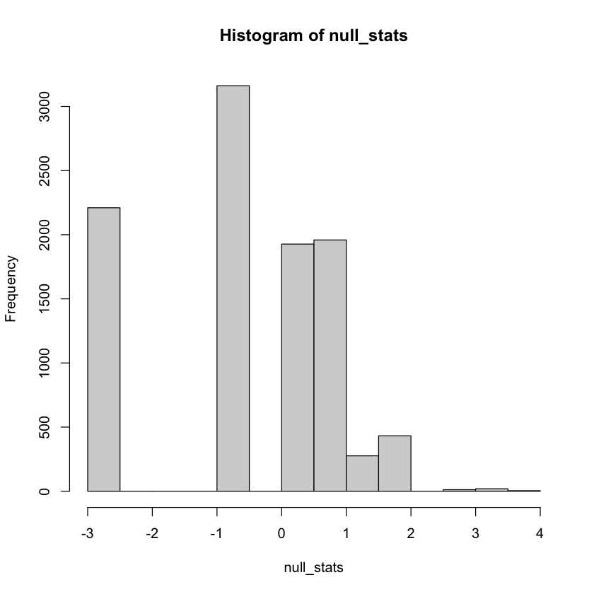
Histogram of \(t\)-statistic under \(H_0\)#
Doesn’t look \(t\)-shaped at all… but test is valid. Why?
Under \(H_0\): shuffling the response doesn’t change the distribution!
hist(null_stats)

Compute a \(p\)-value#
observed = t.test(Incidents ~ Launch, data=orings)$stat
observed
mean(null_stats > observed)
Rank Sum Test#
One can use any test statistic for permutation test…
Only tests null \(H_0\): distributions are the same.
What should we use for \(H_a\)?
Case study B: difference in cognitive load#
Time to solve math problems under two different presentations
Small sample size, not normal?
cognitive_load = read.csv('https://raw.githubusercontent.com/StanfordStatistics/stats191-data/main/Sleuth3/cognitive_load.csv', header=TRUE)
cognitive_load
| Time | Treatment | Censored |
|---|---|---|
| <int> | <chr> | <int> |
| 68 | Modified | 0 |
| 70 | Modified | 0 |
| 73 | Modified | 0 |
| 75 | Modified | 0 |
| 77 | Modified | 0 |
| 80 | Modified | 0 |
| 80 | Modified | 0 |
| 132 | Modified | 0 |
| 148 | Modified | 0 |
| 155 | Modified | 0 |
| 183 | Modified | 0 |
| 197 | Modified | 0 |
| 206 | Modified | 0 |
| 210 | Modified | 0 |
| 130 | Conventional | 0 |
| 139 | Conventional | 0 |
| 146 | Conventional | 0 |
| 150 | Conventional | 0 |
| 161 | Conventional | 0 |
| 177 | Conventional | 0 |
| 228 | Conventional | 0 |
| 242 | Conventional | 0 |
| 265 | Conventional | 0 |
| 300 | Conventional | 1 |
| 300 | Conventional | 1 |
| 300 | Conventional | 1 |
| 300 | Conventional | 1 |
| 300 | Conventional | 1 |
Rank sum test#
Rank the outcome
\(T\) = Sum the ranks in one of the groups (14 of 28 are
Modified)Under \(H_0:\) distributions are identical, \(T\) has distribution the sum of 14 ranks in a random permutation…
cognitive_load$R = rank(cognitive_load$Time)
rank_sum = with(cognitive_load, sum(R[Treatment == 'Modified']))
rank_sum
W = 14^2 + 14*15/2 - rank_sum
c(W, 14*14-W)
- 164
- 32
Rank sum test#
Using a builtin test
wilcox.test(Time ~ Treatment,
            data=cognitive_load,
            alternative='greater')
Warning message in wilcox.test.default(x = DATA[[1L]], y = DATA[[2L]], ...):
“cannot compute exact p-value with ties”
	Wilcoxon rank sum test with continuity correction

data:  Time by Treatment
W = 164, p-value = 0.001271
alternative hypothesis: true location shift is greater than 0
Rank sum test#
Null distribution (ignoring ties)#
null_sample = runif(28)
null_treat = c(rep('M', 14), rep('U', 14))
null_df = data.frame(S=null_sample, T=null_treat)
null_df$R = rank(null_df$S)
with(null_df, sum(R[T=='M']))
Ruses a distributional approximation…
Confidence interval#
wilcox.test(Time ~ Treatment,
            data=cognitive_load,
            alternative='two.sided',
            conf.int=TRUE)
Warning message in wilcox.test.default(x = DATA[[1L]], y = DATA[[2L]], ...):
“cannot compute exact p-value with ties”
Warning message in wilcox.test.default(x = DATA[[1L]], y = DATA[[2L]], ...):
“cannot compute exact confidence intervals with ties”
	Wilcoxon rank sum test with continuity correction

data:  Time by Treatment
W = 164, p-value = 0.002542
alternative hypothesis: true location shift is not equal to 0
95 percent confidence interval:
  57.00007 159.99998
sample estimates:
difference in location
                    94
What parameter is this estimating?
Shift alternative#
 {height=400 fig-align=”center”}
\(H_a:\) the difference between groups is a simple shift
Other interpretations: estimating median of difference…
Paired data#
There are plenty of other non-parametric tests out there
Signed rank test for paired data (i.e. schizophrenia)#
\(H_0:\) distributions are the same in each group..
\(\implies\) differences are symmetrically distributed around 0!
Symmetric null#
 {height=400 fig-align=”center”}
\(H_0:\) distribution is symmetric around 0.
Symmetric alternative#
 {height=400 fig-align=”center”}
\(H_a:\) distribution is symmetric around \(\delta\).
Example of signed rank schizophrenia#
schizophrenia = read.csv('https://raw.githubusercontent.com/StanfordStatistics/stats191-data/main/Sleuth3/schizophrenia.csv', header=TRUE)
with(schizophrenia, wilcox.test(Affected, Unaffected), paired=TRUE)
Warning message in wilcox.test.default(Affected, Unaffected):
“cannot compute exact p-value with ties”
	Wilcoxon rank sum test with continuity correction

data:  Affected and Unaffected
W = 71.5, p-value = 0.09295
alternative hypothesis: true location shift is not equal to 0
Compare to t.test#
with(schizophrenia, t.test(Affected - Unaffected))
	One Sample t-test

data:  Affected - Unaffected
t = -3.2289, df = 14, p-value = 0.006062
alternative hypothesis: true mean is not equal to 0
95 percent confidence interval:
 -0.3306292 -0.0667041
sample estimates:
 mean of x
-0.1986667
