T distributions#
Download#
Outline#
Case studies:
Volume of left hippocampus in discordant twins (for schizophrenia)
Difference in finches’ beaks before and after drought
Descriptive statistics:
Median
Standard deviation
Median
\(t\)-distributions
One-sample \(t\)-test
Confidence intervals
Two sample \(t\)-test
library(ggplot2)
set.seed(0)
Numerical descriptive statistics#
Mean of a sample#
Given a sample of numbers \(X=(X_1, \dots, X_n)\) the sample mean, \(\overline{X}\) is
Artificial example#
X = c(1,3,5,7,8,12,19)
X
- 1
- 3
- 5
- 7
- 8
- 12
- 19
Lots of ways to compute the mean
(X[1]+X[2]+X[3]+X[4]+X[5]+X[6]+X[7])/7
sum(X)/length(X)
mean(X)
Exercise#
Compute the mean of volume in
Affectedgroup of Schizophrenia study
schizophrenia = read.csv('https://raw.githubusercontent.com/StanfordStatistics/stats191-data/main/Sleuth3/schizophrenia.csv', header=TRUE)
head(schizophrenia)
| Unaffected | Affected | |
|---|---|---|
| <dbl> | <dbl> | |
| 1 | 1.94 | 1.27 |
| 2 | 1.44 | 1.63 |
| 3 | 1.56 | 1.47 |
| 4 | 1.58 | 1.39 |
| 5 | 2.06 | 1.93 |
| 6 | 1.66 | 1.26 |
Standard deviation of a sample#
Given a sample of numbers \(X=(X_1, \dots, X_n)\) the sample standard deviation \(S_X\) is $\( S^2_X = \frac{1}{n-1} \sum_{i=1}^n (X_i-\overline{X})^2.\)$
S2 = sum((X - mean(X))^2) / (length(X)-1)
sqrt(S2)
sd(X)
Exercise#
Compute the standard deviation of volume in
Affectedgroup of Schizophrenia study
Median of a sample#
Given a sample of numbers \(X=(X_1, \dots, X_n)\) the sample median is
the middle of the sample:
if \(n\) is even, it is the average of the middle two points.
If \(n\) is odd, it is the midpoint.
median(X)
median(c(X, 13))
One-sample \(T\)-test#
Suppose we want to determine whether the volume of left hiccomapus in
Affectedvs.Unaffected.Let’s compute the
Differencesof the two
schizophrenia$Differences = (schizophrenia$Unaffected -
                             schizophrenia$Affected)
head(schizophrenia)
| Unaffected | Affected | Differences | |
|---|---|---|---|
| <dbl> | <dbl> | <dbl> | |
| 1 | 1.94 | 1.27 | 0.67 |
| 2 | 1.44 | 1.63 | -0.19 |
| 3 | 1.56 | 1.47 | 0.09 |
| 4 | 1.58 | 1.39 | 0.19 |
| 5 | 2.06 | 1.93 | 0.13 |
| 6 | 1.66 | 1.26 | 0.40 |
The test is performed by estimating the average difference and converting to standardized units.
A mental model for the test#
Formally, could set up the above test as drawing from a box of differences in discordant twins’ volume of left hippocampus.
We can think of the sample of differences as having drawn 15 patients at random from a large population (box) containing all possible such differences.
Under \(H_0\): the average of all possible such differences is 0.
Mental model: population of twins#
 {width=500 fig-align=”center”}
Population: pairs of discordant twins
Mental model: population of twins#
{width=500 fig-align=”center”}
\(H_0\): the average difference between
AffectedandUnaffectedis 0.The alternative hypothesis is \(H_a:\) the average difference is not zero.
Mental model: sampling 15 pairs#
 {width=500 fig-align=”center”}
A sample of 15 pairs of discordant twins
One-sample \(T\)-test#
The test is usually a \(T\) test that uses the statistic
The formula can be read in three parts:
Estimating the mean: \(\overline{X}\)
Comparing to 0: subtracting 0 in the numerator. Why 0?
Converting difference to standardized units: dividing by \(S_X/\sqrt{n}\).
Standard error of \(\bar{X}\)#
The denominator above serves as an estimate of \(SD(\overline{X})\) the *standard deviation of \(\overline{X}\) *.
Carrying out the test#
Compute the \(t\)-statistic#
T = (mean(schizophrenia$Differences) - 0) / (sd(schizophrenia$Differences) / sqrt(15))
T
Compare to 5% cutoff#
cutoff = qt(0.975, 14)
cutoff
Conclusion#
The result of the two-sided test is
reject = (abs(T) > cutoff)
reject
If reject is TRUE, then we reject \(H_0\) the mean is 0 at a level
of 5%, while if it is FALSE we do not reject.
Type I error: what does 5% represent?#
If \(H_0\) is true (\(P \in H_0\)) and some modelling assumptions hold, then
Modelling assumptions#
For us to believe the Type I error to be exactly 5% we should be comfortable assuming that the distribution of
Differencesin the population follows a normal curve.For us to believe the Type I error to be close to 5% we should be comfortable assuming that the distribution of the \(T\)-statistic behaves similarly to as if the data were from a normal curve…
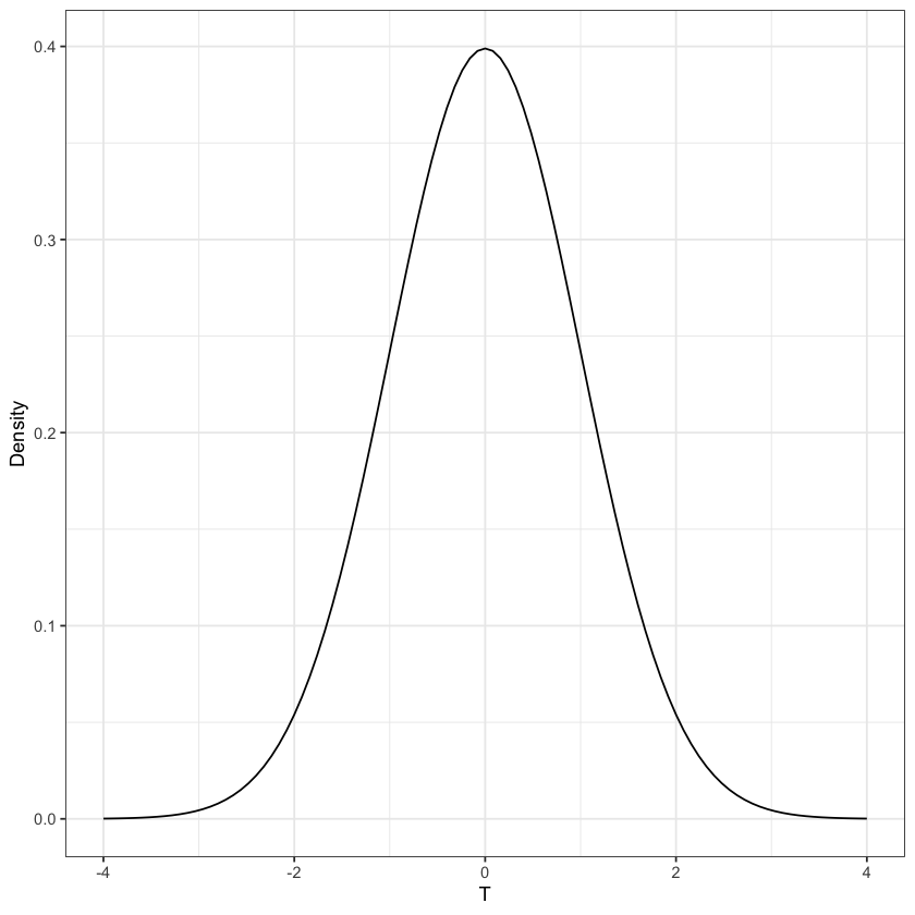
Normal distribution#
Mean=0, Standard deviation=1#
xval = seq(-4,4,length=101)
fig = (ggplot(data.frame(x=xval), aes(x)) +
    stat_function(fun=dnorm, geom='line') +
    labs(y='Density', x='T') +
    theme_bw())
fig
Rejection region for \(T_{14}\)#
alpha = 0.05
df = 14
q = qt(1-alpha/2, df)

rejection_region = function(dens, q_lower, q_upper, xval, fill='#CC7777') {
    fig = (ggplot(data.frame(x=xval), aes(x)) +
        stat_function(fun=dens, geom='line') +
        stat_function(fun=function(x) {ifelse(x > q_upper | x < q_lower, dens(x), NA)},
                    geom='area', fill=fill)  +
        labs(y='Density', x='T') +
        theme_bw())
    return(fig)
}

T14_fig = rejection_region(function(x) { dt(x, df)}, -q, q, xval) +
          annotate('text', x=2.5, y=dt(2,df)+0.3, label='Two sided rejection region, df=14')

T14_fig
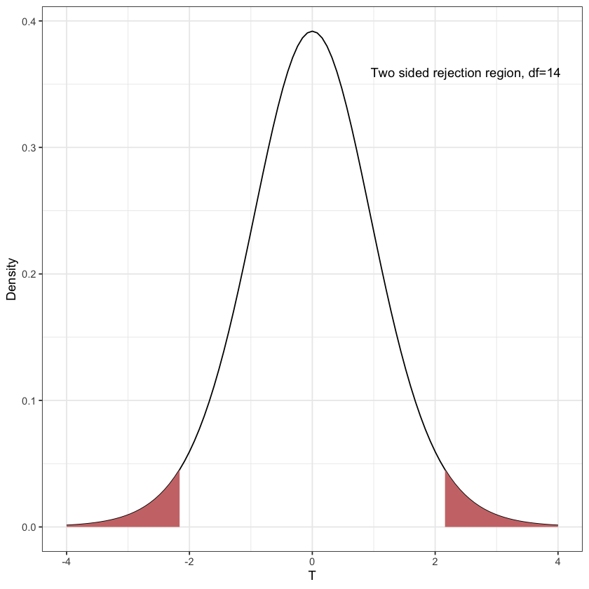
Looks like a normal curve, but heavier tails…
For a test of size \(\alpha\) we write this cutoff \(t_{n-1,1-\alpha/2}\).
Testing the difference of volumes in the Schizophrenia study#
t.test(schizophrenia$Differences)
	One Sample t-test

data:  schizophrenia$Differences
t = 3.2289, df = 14, p-value = 0.006062
alternative hypothesis: true mean is not equal to 0
95 percent confidence interval:
 0.0667041 0.3306292
sample estimates:
mean of x
0.1986667
T
2 * pt(abs(T), 14, lower=FALSE)
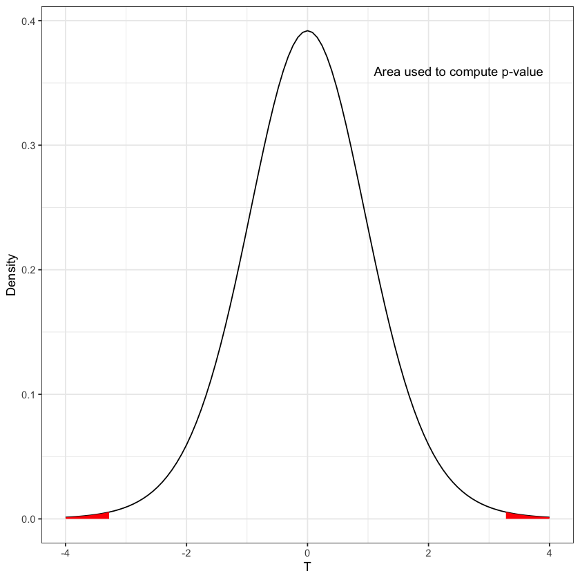
Computation of \(p\)-value#
T = 3.22898
pval_fig = rejection_region(function(x) { dt(x, df)}, -abs(T), abs(T), xval, fill='red') +
            annotate('text', x=2.5, y=dt(2,df)+0.3, label='Area used to compute p-value')
pval_fig
Confidence intervals#
If the 5% cutoff is \(q\) for our test, then the 95% confidence interval is $\( [\bar{X} - q \cdot S_X / \sqrt{n}, \bar{X} + q \cdot S_X / \sqrt{n}] \)\( where we recall \)q=t_{n-1,0.975}\( with \)n=15$.
If we wanted 90% confidence interval, we would use \(q=t_{14,0.95}\). Why?
Computing an interval by hand#
diffs = schizophrenia$Differences
q = qt(0.975, 14)
L = mean(diffs) - q * sd(diffs)/sqrt(15)
U = mean(diffs) + q * sd(diffs)/sqrt(15)
c(L=L, U=U)
- L
- 0.066704104694866
- U
- 0.330629228638467
t.test(diffs)
	One Sample t-test

data:  diffs
t = 3.2289, df = 14, p-value = 0.006062
alternative hypothesis: true mean is not equal to 0
95 percent confidence interval:
 0.0667041 0.3306292
sample estimates:
mean of x
0.1986667
Interpreting confidence intervals#
Let’s suppose the average difference in volume is 0.1
truth = 0.1
hypothetical = rnorm(15) + truth
CI = t.test(hypothetical)$conf.int
CI
cover = (CI[1] < truth) * (CI[2] > truth)
cover
- -0.38647235576234
- 0.828804375364375
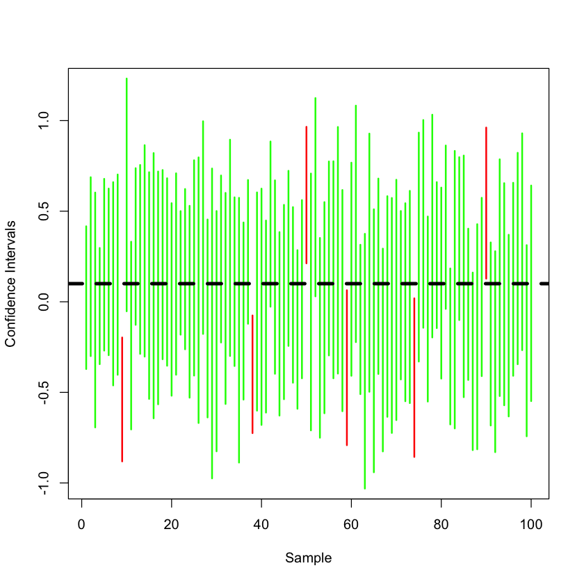
Generating 100 versions of CI#
A useful picture is to plot all these intervals so we can see the randomness in the intervals, while the true mean of the box is unchanged.
truth = 0.1
plot(c(1, 100), c(-1.1+truth,1.1+truth), type='n', ylab='Confidence Intervals', xlab='Sample')
for (i in 1:100) {
    hypothetical = rnorm(15) + truth
    CI = t.test(hypothetical)$conf.int
    cover = (CI[1] < truth) * (CI[2] > truth)
    cover
   if (cover == TRUE) {
       lines(c(i,i), c(CI[1],CI[2]), col='green', lwd=2)
   }
   else {
      lines(c(i,i), c(CI[1],CI[2]), col='red', lwd=2)
   }
}
abline(h=truth, lty=2, lwd=4)
Case Study: beak depths#
Is there a change in the finches’ beak depth after the drought in 1977?
beaks = read.csv('https://raw.githubusercontent.com/StanfordStatistics/stats191-data/main/Sleuth3/beaks.csv', header=TRUE)
beaks$Year = factor(beaks$Year)
head(beaks)
| Year | Depth | |
|---|---|---|
| <fct> | <dbl> | |
| 1 | 1976 | 6.2 |
| 2 | 1976 | 6.8 |
| 3 | 1976 | 7.1 |
| 4 | 1976 | 7.1 |
| 5 | 1976 | 7.4 |
| 6 | 1976 | 7.8 |
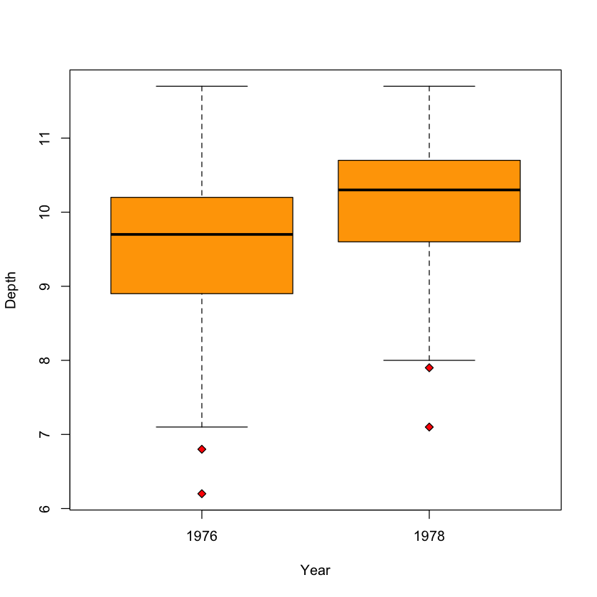
Boxplots#
boxplot(Depth ~ Year,
        data=beaks,
        col='orange',
        pch=23,
        bg='red')
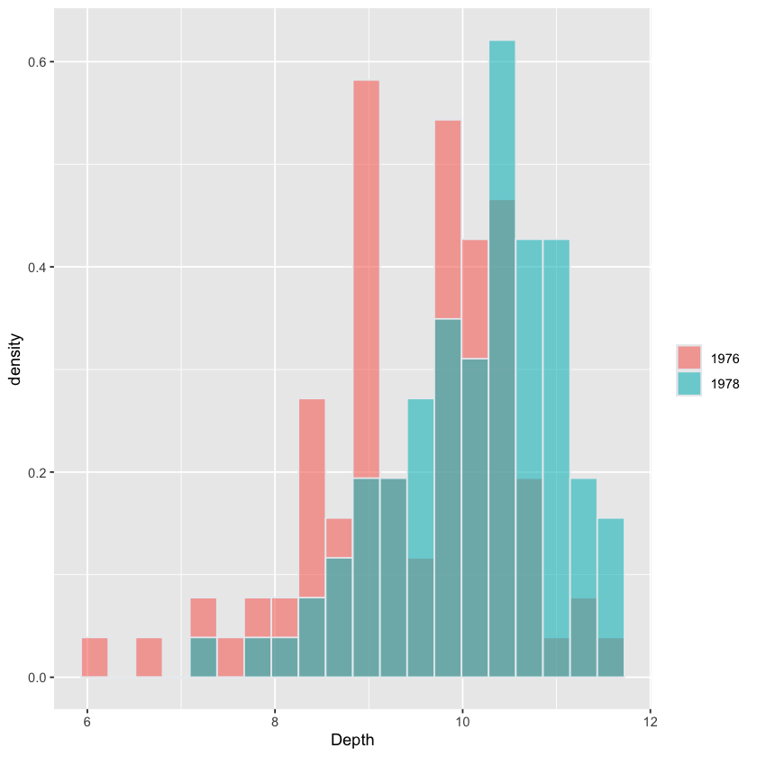
Histogram of Depth stratified by Year#
# this plot is for visualization only
# students not expected to reproduce

beaks = read.csv('https://raw.githubusercontent.com/StanfordStatistics/stats191-data/main/Sleuth3/beaks.csv', header=TRUE)
beaks$Year = factor(beaks$Year)
fig <- (ggplot(beaks, aes(x=Depth, fill=Year)) +
        geom_histogram(aes(y=after_stat(density)),
                       color="#e9ecef",
	               alpha=0.6,
		       position='identity',
		       bins=20) +
        labs(fill=""))
fig
Mental model: two samples#
 {width=500 fig-align=”center”}
Two populations of finches (
1976and1978)
Two-sample \(t\)-test#
We have two samples:
\((B_1, \dots, B_{89})\) (before,
1976)\((A_1, \dots, A_{89})\) (after,
1978)
Model:
We can answer this statistically by testing the null hypothesis \(H_0:\mu_B = \mu_A.\)
Pooled \(t\)-test#
If variances are equal \((\sigma^2_A=\sigma^2_B)\), the pooled \(t\)-test is appropriate.
The test statistic is
Form of the \(t\)-statistic#
The parts of the \(t\)-statistic are similar to the one-sample case:
Estimate of our parameter: \(\overline{A} - \overline{B}\): our estimate of \(\mu_A-\mu_B\)
Compare to 0 (we are testing \(H_0:\mu_A-\mu_B=0\))
Convert to standard units (formula is different, reason is the same)
Interpreting the results#
For two-sided test at level \(\alpha=0.05\), reject if \(|T| > t_{176, 0.975}\).
Confidence interval: for example, a \(90\%\) confidence interval for \(\mu_A-\mu_B\) is
Carrying out the test#
B = beaks$Depth[beaks$Year==1976]
A = beaks$Depth[beaks$Year==1978]
sdP = sqrt((88*sd(A)^2 + 88*sd(B)^2)/176)
T = (mean(A)-mean(B)-0) / (sdP * sqrt(1/89+1/89))
c(T=T, cutoff=qt(0.975, 176))
- T
- 4.58327601981588
- cutoff
- 1.9735343877061
Using R#
Rhas a builtin function to perform such \(t\)-tests.
t.test(Depth ~ Year, data=beaks, var.equal=TRUE)
	Two Sample t-test

data:  Depth by Year
t = -4.5833, df = 176, p-value = 8.65e-06
alternative hypothesis: true difference in means between group 1976 and group 1978 is not equal to 0
95 percent confidence interval:
 -0.9564088 -0.3806698
sample estimates:
mean in group 1976 mean in group 1978
          9.469663          10.138202
Unequal variance#
If we don’t make the assumption of equal variance,
Rwill give a slightly different result.More on this in Chapter 4.
t.test(Depth ~ Year, data=beaks)
	Welch Two Sample t-test

data:  Depth by Year
t = -4.5833, df = 172.98, p-value = 8.739e-06
alternative hypothesis: true difference in means between group 1976 and group 1978 is not equal to 0
95 percent confidence interval:
 -0.9564436 -0.3806350
sample estimates:
mean in group 1976 mean in group 1978
          9.469663          10.138202
Pooled estimate of variance#
The rule for the \(SD\) of differences is $\( SD(\overline{A}-\overline{B}) = \sqrt{SD(\overline{A})^2+SD(\overline{B})^2}\)$
By this rule, we might take our estimate to be $\( SE(\overline{A}-\overline{B}) = \widehat{SD(\overline{A}-\overline{B})} = \sqrt{\frac{S^2_A}{89} + \frac{S^2_B}{89}}. \)$
The pooled estimate assumes \(E(S^2_A)=E(S^2_B)=\sigma^2\) and replaces the \(S^2\)’s above with \(S^2_P\), a better estimate of n \(\sigma^2\) than either \(S^2_A\) or \(S^2_B\).
Where do we get \(df=176\)?#
The \(A\) sample has \(89-1=88\) degrees of freedom to estimate \(\sigma^2\) while the \(B\) sample also has \(89-1=88\) degrees of freedom.
Therefore, the total degrees of freedom is \(88+88=176\).
Our first regression model#
We can put the two samples together: $\(Y=(A_1,\dots, A_{89}, B_1, \dots, B_{89}).\)$
Under the same assumptions as the pooled \(t\)-test: $\( \begin{aligned} Y_i &\sim N(\mu_i, \sigma^2)\\ \mu_i &= \begin{cases} \mu_A & 1 \leq i \leq 89 \\ \mu_B & 90 \leq i \leq 178. \end{cases} \end{aligned} \)$
Features and responses#
This is a regression model for the sample \(Y\). The (qualitative) variable
Yearis called a covariate or predictor.The
Depthis the outcome or response.We assume that the relationship between
DepthandYearis simple: it depends only on which group a subject is in.This relationship is modelled through the mean vector \(\mu=(\mu_1, \dots, \mu_{178})\).
A little look ahead#
Let’s carry out our test by fitting our regression model with
lm:
sdP * sqrt(1/89 + 1/89)
sdP
summary(lm(Depth ~ Year, data=beaks))
Call:
lm(formula = Depth ~ Year, data = beaks)

Residuals:
    Min      1Q  Median      3Q     Max
-3.2697 -0.5382  0.1618  0.6303  2.2303

Coefficients:
            Estimate Std. Error t value Pr(>|t|)
(Intercept)   9.4697     0.1031  91.812  < 2e-16 ***
Year1978      0.6685     0.1459   4.583 8.65e-06 ***
---
Signif. codes:  0 ‘***’ 0.001 ‘**’ 0.01 ‘*’ 0.05 ‘.’ 0.1 ‘ ’ 1

Residual standard error: 0.973 on 176 degrees of freedom
Multiple R-squared:  0.1066,	Adjusted R-squared:  0.1016
F-statistic: 21.01 on 1 and 176 DF,  p-value: 8.65e-06