Diagnostics II#
Download#
Gesell Score Data Set {.scrollable}#
The Gesell score is used to measure child development.
How does it correlate with the age (in months) at which a child speaks their first word?
df.child <- read.csv("https://dlsun.github.io/data/gesell.csv")
head(df.child)
| AgeAtFirstWord | GesellScore | |
|---|---|---|
| <int> | <int> | |
| 1 | 15 | 95 |
| 2 | 26 | 71 |
| 3 | 10 | 83 |
| 4 | 9 | 91 |
| 5 | 15 | 102 |
| 6 | 20 | 87 |
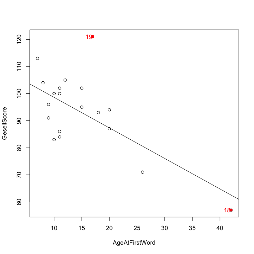
Influential Points#
Which point do you think has the most “influence” on the fitted regression line?
#| echo: false
df.child <- read.csv("https://dlsun.github.io/data/gesell.csv")
with(df.child, {
  plot(AgeAtFirstWord, GesellScore);
  abline(lm(GesellScore ~ AgeAtFirstWord));
  points(AgeAtFirstWord[18:19], GesellScore[18:19], col="red", pch=15);
  text(AgeAtFirstWord[18:19] - 0.7, GesellScore[18:19], labels=18:19, col="red")
})
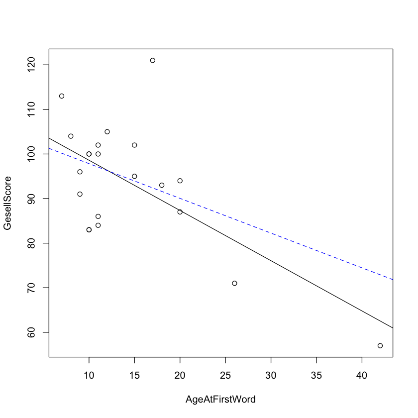
Influential Points {.scrollable}#
Let’s try deleting each point and seeing which one changes the regression line more.
with(df.child, plot(AgeAtFirstWord, GesellScore))
abline(lm(GesellScore ~ AgeAtFirstWord, data=df.child))
abline(lm(GesellScore ~ AgeAtFirstWord, data=df.child[-18, ]),
       lty=2, col="blue")
Measuring Influence#
How do we quantify how much “influence” a point has on the regression line?
Mathematical Detour: The Hat Matrix#
In thinking about influence, it is helpful to note that each fitted value \(\hat Y_i\) can be expressed as a weighted sum of the \(Y\) values:
…
Collectively, the weights \(h_{ij}\) make up a matrix \(H\).
…
\(H\) is called the “hat matrix” because it puts the “hat” on \(Y\).
Diagnostic 1: Leverage#
The leverage of an observation is the weight \(h_{ii}\) that observation \(i\) assigns to its own \(Y\) value.
::: {.incremental}
For simple linear regression, there is an easy formula \(h_{ii}\): $\( h_{ii} = \frac{(X_i - \bar X)^2}{\sum_i (X_i - \bar X)^2} + \frac{1}{n}. \)$
For multiple regression, the formula requires matrix algebra. :::
…
Either way, leverage measures how far observation \(i\) is from the average, in the explanatory variables.
Diagnostic 1: Leverage {.smaller .scrollable}#
In R, the hatvalues function calculates the leverage of each observation.
model <- lm(GesellScore ~ AgeAtFirstWord, data=df.child)
hatvalues(model)
- 1
- 0.0479224794510218
- 2
- 0.154513234296056
- 3
- 0.0628157755825353
- 4
- 0.0705452077520549
- 5
- 0.0479224794510218
- 6
- 0.0726189578463163
- 7
- 0.0579895935449815
- 8
- 0.0566699343940879
- 9
- 0.0798582309026469
- 10
- 0.0726189578463163
- 11
- 0.0907548450343111
- 12
- 0.0705452077520549
- 13
- 0.0628157755825353
- 14
- 0.0566699343940879
- 15
- 0.0566699343940879
- 16
- 0.0628157755825353
- 17
- 0.0521076841867129
- 18
- 0.65160998416409
- 19
- 0.0530502978659226
- 20
- 0.0566699343940879
- 21
- 0.0628157755825353
…
Observation 18 has the highest leverage by far. This is no surprise because it had a very large \(X\) value.
…
Some Properties of Leverage
::: {.incremental}
\(\frac{1}{n} \leq h_{ii} < 1\)
\(\sum_i h_{ii} = p + 1\) (number of coefficients including the intercept), so the average leverage is \(\bar h = \frac{p + 1}{n}\).
Some books recommend flagging observations with \(h_{ii} > 2\bar h = 2\frac{p + 1}{n}\). :::
Diagnostic 2: DFFIT#
Maybe we need a metric that looks more directly at how much the prediction changes when we delete observation \(i\).
…
We compare the following predictions:
\(\hat Y\): predicted values from a model fit to all observations.
\(\hat Y^{(-i)}\): predicted values from a model fit to all observations, except observation \(i\).
…
A reasonable diagnostic is the “difference in fits”:
Diagnostic 2: DFFIT {.scrollable}#
There is no built-in function to calculate DFFIT. (The function dffits
calculates a studentized version called DFFITS.)
…
However, it is not hard to implement DFFIT from scratch.
i <- 18
model1 <- lm(GesellScore ~ AgeAtFirstWord, data=df.child)
model2 <- lm(GesellScore ~ AgeAtFirstWord, data=df.child[-i, ])
model1$fitted[i] - model2$fitted[i]
Diagnostic 3: Cook’s Distance {.smaller}#
:::: {.columns}
::: {.column width=”30%”}

Dennis Cook (1944 - )
Professor of Statistics, University of Minnesota :::
::: {.column width=”70%”} Cook’s distance measures how much the predictions for all \(n\) observations change, when observation \(i\) is deleted:
::: {.fragment} Fortunately, this can be calculated without refitting the model each time a different observation is deleted. An equivalent formula is:
:::
::: ::::
Diagnostic 3: Cook’s Distance {.scrollable}#
In R, the cooks.distance function calculates the Cook’s distance of each observation.
cooks.distance(model)
- 1
- 0.000897406392870688
- 2
- 0.0814979551507635
- 3
- 0.0716581442213833
- 4
- 0.0256159582452641
- 5
- 0.0177436626335013
- 6
- 3.87762740910136e-05
- 7
- 0.0031305748029949
- 8
- 0.00166820857813469
- 9
- 0.00383194880672965
- 10
- 0.0154395158127621
- 11
- 0.0548101351203612
- 12
- 0.00467762256482441
- 13
- 0.0716581442213833
- 14
- 0.0475978118328145
- 15
- 0.00536121617564154
- 16
- 0.000573584529113046
- 17
- 0.017856495213809
- 18
- 0.678112028575845
- 19
- 0.223288273631179
- 20
- 0.0345188940892692
- 21
- 0.000573584529113046
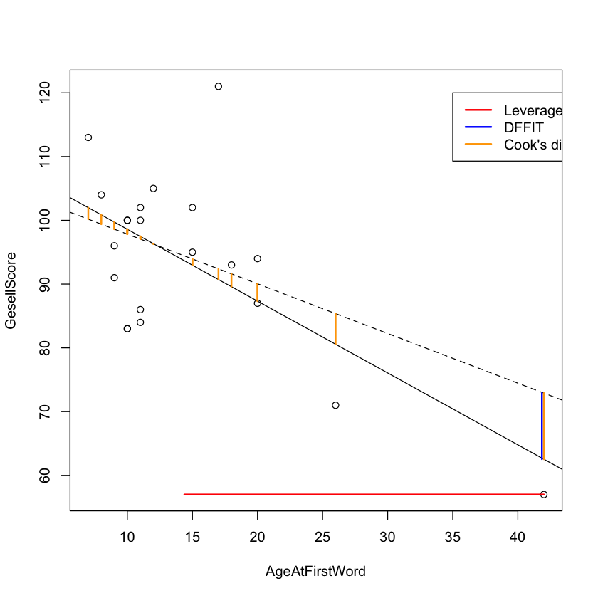
Visual Comparison of Diagnostics#
#| echo: false
with(df.child, plot(AgeAtFirstWord, GesellScore))

model1 <- lm(GesellScore ~ AgeAtFirstWord, data=df.child)
model2 <- lm(GesellScore ~ AgeAtFirstWord, data=df.child[-18, ])

abline(model1)
abline(model2, lty=2)

arrows(df.child$AgeAtFirstWord[18], df.child$GesellScore[18],
       mean(df.child$AgeAtFirstWord), df.child$GesellScore[18],
       col="red", code=0, lwd=2)
arrows(df.child$AgeAtFirstWord[18] - 0.15, model1$fitted[18],
       df.child$AgeAtFirstWord[18] - 0.15, predict(model2, df.child)[18],
       col="blue", code=0, lwd=2)

for(i in 1:nrow(df.child)) {
  arrows(df.child$AgeAtFirstWord[i], model1$fitted[i],
         df.child$AgeAtFirstWord[i], predict(model2, df.child)[i],
         col="orange", code=0, lwd=2)
}

legend(x=35, y=120,
       legend=c("Leverage", "DFFIT", "Cook's distance"), col=c("red", "blue", "orange"),
       lty=c(1, 1, 1), lwd=c(2, 2, 2))
Putting It All Together {.scrollable}#
R provides a function, influence.measures, that calculates these diagnostics
and more.
influence.measures(model)
Influence measures of
	 lm(formula = GesellScore ~ AgeAtFirstWord, data = df.child) :

     dfb.1_ dfb.AAFW    dffit cov.r   cook.d    hat inf
1   0.01664  0.00328  0.04127 1.166 8.97e-04 0.0479
2   0.18862 -0.33480 -0.40252 1.197 8.15e-02 0.1545
3  -0.33098  0.19239 -0.39114 0.936 7.17e-02 0.0628
4  -0.20004  0.12788 -0.22433 1.115 2.56e-02 0.0705
5   0.07532  0.01487  0.18686 1.085 1.77e-02 0.0479
6   0.00113 -0.00503 -0.00857 1.201 3.88e-05 0.0726
7   0.00447  0.03266  0.07722 1.170 3.13e-03 0.0580
8   0.04430 -0.02250  0.05630 1.174 1.67e-03 0.0567
9   0.07907 -0.05427  0.08541 1.200 3.83e-03 0.0799
10 -0.02283  0.10141  0.17284 1.152 1.54e-02 0.0726
11  0.31560 -0.22889  0.33200 1.088 5.48e-02 0.0908
12 -0.08422  0.05384 -0.09445 1.183 4.68e-03 0.0705
13 -0.33098  0.19239 -0.39114 0.936 7.17e-02 0.0628
14 -0.24681  0.12536 -0.31367 0.992 4.76e-02 0.0567
15  0.07968 -0.04047  0.10126 1.159 5.36e-03 0.0567
16  0.02791 -0.01622  0.03298 1.187 5.74e-04 0.0628
17  0.13328 -0.05493  0.18717 1.096 1.79e-02 0.0521
18  0.83112 -1.11275 -1.15578 2.959 6.78e-01 0.6516   *
19  0.14348  0.27317  0.85374 0.396 2.23e-01 0.0531   *
20 -0.20761  0.10544 -0.26385 1.043 3.45e-02 0.0567
21  0.02791 -0.01622  0.03298 1.187 5.74e-04 0.0628
How to Deal with Influential Observations#

Measuring Outliers#
Even if observation 19 is not influential, it still has a large residual, so it may be an outlier.
How do we detect outliers?
Studentized Residual {.smaller}#
Recall the difference between \(z\) and \(t\) statistics. (See Sleuth, Chapter 2.2.3.)
:::: {.columns} ::: {.column width=”50%”} $\( z = \frac{\text{estimate} - \text{parameter}}{\text{SD(estimate)}} \)$
Dividing by the SD is called standardization.
::: ::: {.column width=”50%”} $\( t = \frac{\text{estimate} - \text{parameter}}{\text{SE(estimate)}} \)$
Dividing by the SE is called studentization. ::: ::::
…
What would a \(t\)-statistic for residuals look like?
::: {.incremental}
Residuals have mean \(0\).
Residuals have SD \(\sigma\sqrt{1 - h_{ii}}\). :::
…
So the studentized residuals are \(\displaystyle t_i = \frac{\text{residual}_i - 0}{\hat\sigma\sqrt{1 - h_{ii}}}\).
A Test for Outliers#
Under the null hypothesis that observation \(i\) comes from the model (i.e., is not an outlier), \(t_i\) should follow a \(t\)-distribution.
::: {.incremental}
For this reason, some books recommend flagging observation \(i\) as an outlier if \(|t_i| > 2\), since \(t_{n-1}(.975) \approx 2\).
But this ignores the fact that any one of the \(n\) observations could be an outlier! The familywise error rate is \(\gg .05\).
We can use the Bonferroni correction. Test each observation at \(\alpha = .05 / n\) so that the familywise error rate is \(\leq .05\). :::
Is Observation 19 an Outlier? {.smaller .scrollable}#
First, let’s calculate the studentized residual $\( t_{19} = \frac{\text{residual}_{19} - 0}{\hat\sigma\sqrt{1 - h_{19,19}}}. \)$
stud.res <- (model$resid[19] /
             (summary(model)$sigma * sqrt(1 - hatvalues(model)[19])))
stud.res
…
Although this appears significant, we should account for the fact that there are 21 observations and any one of them could be an outlier. The actual cutoff we should use is:
n <- 21
alpha <- .05 / n
qt(1 - alpha / 2, df=n - 1)
Summary#
Influential Points
Leverage
DFFIT
Cook’s distance
Outliers
Studentized residual can be used as an outlier test, but need to be careful about multiple testing.