ANOVA

Download

• Slides

• RStudio: RMarkdown,Quarto

• Jupyter

Outline

• ANOVA models: variables with only categorical variables

• Case studies:

  A. Seaweed regeneration time based on grazers

  B. Pygmalion effect

Case study A: Seaweed grazers

url = 'https://raw.githubusercontent.com/StanfordStatistics/stats191-data/main/Sleuth3/seaweed_grazers.csv'
seaweed.df = read.csv(url, sep=',', header=TRUE)
head(seaweed.df)

A data.frame: 6 × 3

	Cover	Block	Treat
	<int>	<chr>	<chr>
1	14	B1	C
2	23	B1	C
3	22	B2	C
4	35	B2	C
5	67	B3	C
6	82	B3	C

• Treat: which animals were allowed into graze

• Block: which of 8 blocks measured

• Cover: what percentage of each block had seaweed covered at time of measurement

Case study B: Pygmalion effect

url = 'https://raw.githubusercontent.com/StanfordStatistics/stats191-data/main/Sleuth3/pygmalion.csv'
pygmalion.df = read.csv(url, sep=',', header=TRUE)
head(pygmalion.df)

A data.frame: 6 × 3

	Company	Treat	Score
	<chr>	<chr>	<dbl>
1	C1	Pygmalion	80.0
2	C1	Control	63.2
3	C1	Control	69.2
4	C2	Pygmalion	83.9
5	C2	Control	63.1
6	C2	Control	81.5

• Company: ID of company

• Treat: whether Pygmalion or Control

• Score: outcome of interest

Additive model

pygm_add.lm = lm(Score ~ Treat + Company, data=pygmalion.df)
anova(pygm_add.lm)

A anova: 3 × 5

	Df	Sum Sq	Mean Sq	F value	Pr(>F)
	<int>	<dbl>	<dbl>	<dbl>	<dbl>
Treat	1	327.3410	327.34102	7.568540	0.01314152
Company	9	682.5171	75.83524	1.753407	0.14844454
Residuals	18	778.5039	43.25022	NA	NA

Saturated model

pygm_sat.lm = lm(Score ~ Treat + Company + Treat:Company, data=pygmalion.df)
anova(pygm_sat.lm)

A anova: 4 × 5

	Df	Sum Sq	Mean Sq	F value	Pr(>F)
	<int>	<dbl>	<dbl>	<dbl>	<dbl>
Treat	1	327.3410	327.34102	6.3079589	0.03322533
Company	9	682.5171	75.83524	1.4613676	0.29050766
Treat:Company	9	311.4639	34.60710	0.6668892	0.72211560
Residuals	9	467.0400	51.89333	NA	NA

Graphical check of additivity

with(pygmalion.df, 
   interaction.plot(Company, Treat, Score,
                    type='p',
                    col=c('red', 'blue'),
		    lwd=2))

Two-way ANOVA model

• Generalization of \(t\)-test: more than one grouping variable.

• Two-way ANOVA model:

  • \(r=8\) groups in first factor (Block)

  • \(m=6\) groups in second factor (Treat)

  • \(n_{ij}\) in each combination of factor variables.

• Model: $\(Y_{ijk} = \mu + \alpha_i + \beta_j + (\alpha \beta)_{ij} + \varepsilon_{ijk} , \qquad \varepsilon_{ijk} \sim N(0, \sigma^2).\)$

• In seaweed.df, \(r=8\), \(m=6\), \(n_{ij}=2\) for all \((i,j)\).

Parameterization

• Some constraints are needed, again for identifiability. Let’s not worry too much about the details…

• Constraints:

  • \(\sum_{i=1}^r \alpha_i = 0\)

  • \(\sum_{j=1}^m \beta_j = 0\)

  • \(\sum_{j=1}^m (\alpha\beta)_{ij} = 0, 1 \leq i \leq r\)

  • \(\sum_{i=1}^r (\alpha\beta)_{ij} = 0, 1 \leq j \leq m.\)

ANOVA table

Source	df	E(MS)
A	r-1	\(\sigma^2 + nm\frac{\sum_{i=1}^r \alpha_i^2}{r-1}\)
B	m-1	\(\sigma^2 + nr\frac{\sum_{j=1}^m \beta_j^2}{m-1}\)
A:B	(m-1)(r-1)	\(\sigma^2 + n\frac{\sum_{i=1}^r\sum_{j=1}^m (\alpha\beta)_{ij}^2}{(r-1)(m-1)}\)
Error	(n-1)mr	\(\sigma^2\)

Tests using the ANOVA table

• Rows of the ANOVA table can be used to test various of the hypotheses we started out with.

• Under \(H_0:\) no interactions

\[F = \frac{MSAB}{MSE} = \frac{\frac{SSAB}{(m-1)(r-1)}}{\frac{SSE}{(n-1)mr}} \sim F_{(m-1)(r-1), (n-1)mr}\]

Test of additivity

• \(H_0\): pygm_add.lm is the true model

anova(pygm_add.lm, pygm_sat.lm)

A anova: 2 × 6

	Res.Df	RSS	Df	Sum of Sq	F	Pr(>F)
	<dbl>	<dbl>	<dbl>	<dbl>	<dbl>	<dbl>
1	18	778.5039	NA	NA	NA	NA
2	9	467.0400	9	311.4639	0.6668892	0.7221156

• \(F\)-statistic \(\approx 0.67\) – very little evidence against \(H_0\).

• Note: this \(F\)-statistic also appears in anova(pygm_sat.lm).

Case study A: seaweed regeneration

seaweed.df$Block = factor(seaweed.df$Block, levels=c('B1','B2','B7','B5', 'B8', 'B6', 'B3', 'B4'))

• Before calling interaction.plot we’ll order Block as book does for Fig 13.9: ordered by total response.

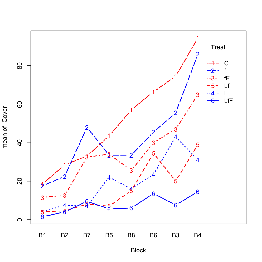
Interaction plot for seaweed

with(seaweed.df,
   interaction.plot(Block, Treat, Cover,
                    type='b',
                    col=c('red', 'blue'),
		    lwd=2))

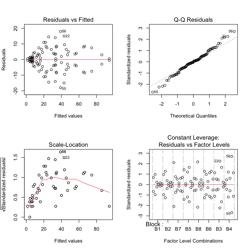
No transformation

seaweed_sat.lm = lm(Cover ~ Block + Treat + Treat:Block, data=seaweed.df)
par(mfrow=c(2,2))
plot(seaweed_sat.lm)

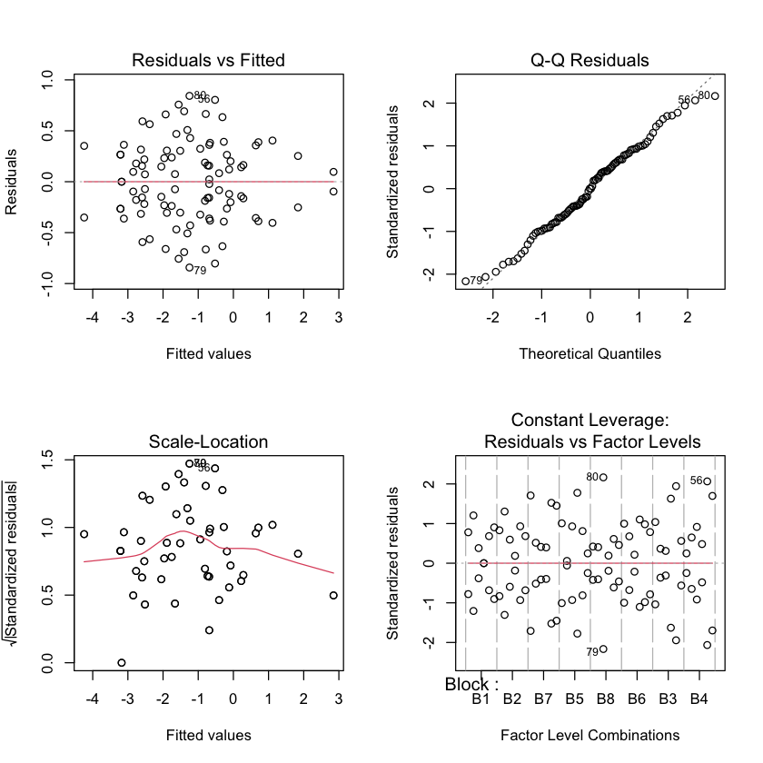
logit transformed

seaweed.df$lCover = with(seaweed.df, log(Cover / (100 - Cover)))
seaweed_lsat.lm = lm(lCover ~ Block + Treat + Treat:Block, data=seaweed.df)
par(mfrow=c(2,2))
plot(seaweed_lsat.lm)

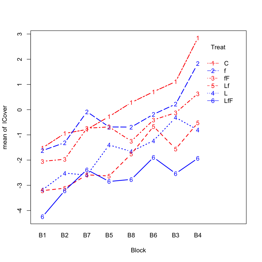
Interaction plot for logit transformed data

with(seaweed.df,
   interaction.plot(Block, Treat, lCover,
                    type='b',
                    col=c('red', 'blue'),
		    lwd=2))

ANOVA table

anova(seaweed_lsat.lm)

A anova: 4 × 5

	Df	Sum Sq	Mean Sq	F value	Pr(>F)
	<int>	<dbl>	<dbl>	<dbl>	<dbl>
Block	7	76.23861	10.8912304	35.963371	5.390313e-17
Treat	5	96.99322	19.3986445	64.055265	4.510728e-20
Block:Treat	35	15.23041	0.4351546	1.436902	1.209129e-01
Residuals	48	14.53643	0.3028423	NA	NA

Another test for Treat

seaweed_ladd.lm = lm(lCover ~ Block + Treat, data=seaweed.df)
anova(seaweed_ladd.lm)

A anova: 3 × 5

	Df	Sum Sq	Mean Sq	F value	Pr(>F)
	<int>	<dbl>	<dbl>	<dbl>	<dbl>
Block	7	76.23861	10.8912304	30.36843	2.133837e-20
Treat	5	96.99322	19.3986445	54.08997	1.094513e-24
Residuals	83	29.76684	0.3586366	NA	NA

• Difference between the two \(F\)-statistics: estimate of \(\sigma^2\)

Inference about specific linear combinations

Do large fish have an effect on the regeneration ratio? If so, how much? (see Display 13.13)

linear_comb = 0 * coef(seaweed_ladd.lm)
linear_comb['TreatLfF'] = 0.5
linear_comb['TreatfF'] = 0.5
linear_comb['TreatLf'] = -0.5
linear_comb['Treatf'] = -0.5
estimate = sum(linear_comb * coef(seaweed_ladd.lm))

Standard error

var_est = sum(linear_comb * (vcov(seaweed_ladd.lm) %*% linear_comb))
SE = sqrt(var_est)
T_stat = estimate / SE
pval = 2 * pt(abs(T_stat), seaweed_ladd.lm$df.resid, lower=FALSE)
c(estimate=estimate, T_stat=T_stat, SE=SE, pval=pval)

estimate

-0.614025727666025

T_stat

-4.10127815915699

SE

0.149715699310733

pval

9.53986852987613e-05

Some caveats about R formulae

While we see that it is straightforward to form the interactions test using our usual anova function approach, we generally cannot test for main effects by this approach.

lm1 = lm(lCover ~ Treat + Block:Treat, data=seaweed.df)
anova(lm1, seaweed_lsat.lm)

A anova: 2 × 6

	Res.Df	RSS	Df	Sum of Sq	F	Pr(>F)
	<dbl>	<dbl>	<dbl>	<dbl>	<dbl>	<dbl>
1	48	14.53643	NA	NA	NA	NA
2	48	14.53643	0	-1.065814e-14	NA	NA

sum((resid(lm1) - resid(seaweed_lsat.lm))^2)

6.59262517602417e-28