Penalized#
Download#
Bias-variance tradeoff#
One goal of a regression analysis is to “build” a model that predicts well – AIC / \(C_p\) & Cross-validation selection criteria based on this.
This is slightly different than the goal of making inferences about \(\beta\) that we’ve focused on so far.
What does “predict well” mean?
Can we take an estimator for a model \({\cal M}\) and make it better in terms of \(MSE\)?
Shrinkage estimators: one sample problem#
Let’s restrict to
Y~1model:
Instead of \(\hat{\mu}=\bar{Y}\) as an estimate of \(\mu\) we’ll use
We shrink the sample mean towards 0!
A little simulation#
Generate \(Y_{100 \times 1} \sim N(\mu \cdot 1, 5^2 I_{100 \times 100})\), with \(\mu=0.5\).
For \(0 \leq \alpha \leq 1\), set \(\hat{\mu}_{\alpha} = \alpha \cdot \bar{Y}.\)
Compute \(MSE(\hat{\mu}_{\alpha}) = \frac{1}{100}\sum_{i=1}^{100} (\hat{\mu}_{\alpha} - 0.5)^2\)
Repeat 1000 times, plot average of \(MSE(\hat{\mu}_{\alpha})\).
For what value of \(\alpha\) is \(\hat{\mu}_{\alpha}\) unbiased?
Is this the best estimate of \(\mu\) in terms of MSE?
mu = 0.5
sigma = 5
nsample = 100
ntrial = 1000

MSE = function(mu.hat, mu) {
  return(sum((mu.hat - mu)^2) / length(mu))
}
alpha = seq(0,1,length=20)
mse = numeric(length(alpha))
bias = (1 - alpha) * mu
variance = alpha^2 * 25 / 100

for (i in 1:ntrial) {
  Z = rnorm(nsample) * sigma + mu
  for (j in 1:length(alpha)) {
    mse[j] = mse[j] + MSE(alpha[j] * mean(Z) * rep(1, nsample), mu * rep(1, nsample))
  }
}
mse = mse / ntrial
Mean-squared error#
plot(alpha, mse, type='l', lwd=2, col='red', ylim=c(0, max(mse)),
     xlab=expression(paste('Shrinkage factor,', alpha)),
     ylab=expression(paste('MSE(', alpha, ')')),
     cex.lab=1.2)
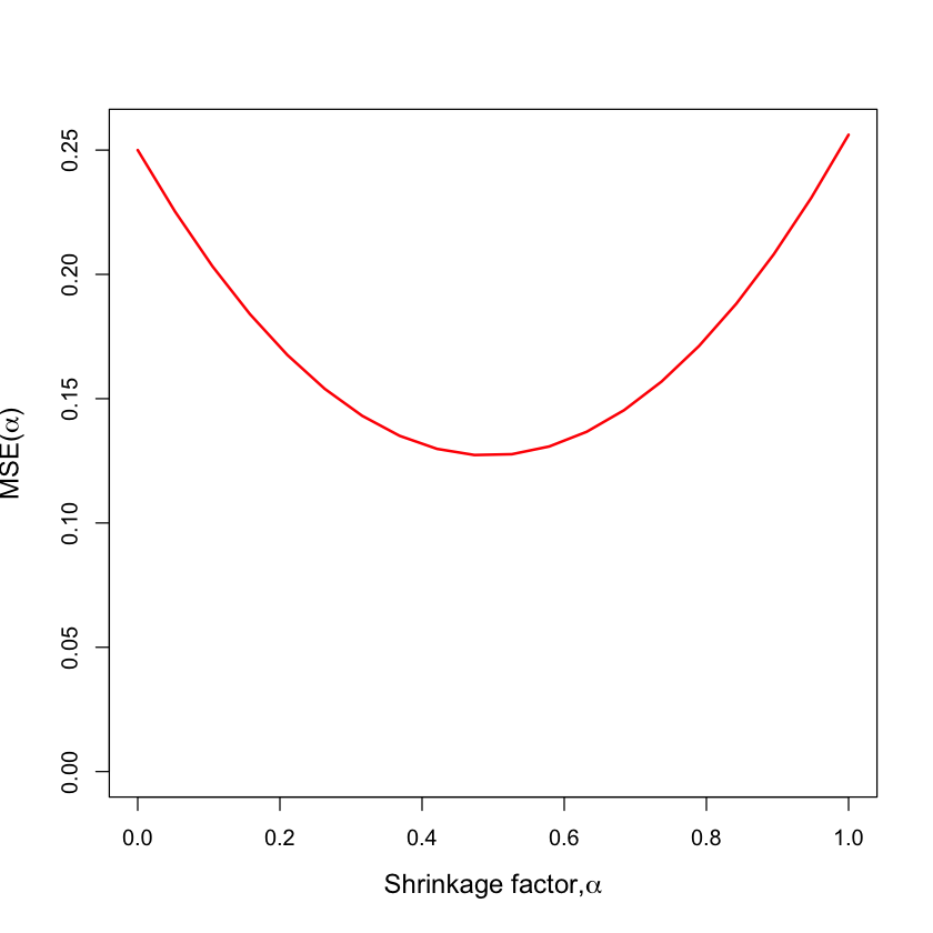
\(\text{E[MSE]}\)
Bias and variance#
plot(alpha, mse, type='l', lwd=2, col='red', ylim=c(0, max(mse)),
     xlab=expression(paste('Shrinkage factor,', alpha)),
     ylab=expression(paste('MSE(', alpha, ')')),
     cex.lab=1.2)
lines(alpha, bias^2, col='green', lwd=2)
lines(alpha, variance, col='blue', lwd=2)
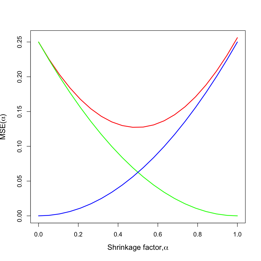
\(\text{Bias}^2\)
\(\text{Variance}\)
\(\text{E[MSE]}\)
Shrinkage & Penalties#
Shrinkage can be thought of as “constrained” or “penalized” minimization.
Constrained form:
Lagrange multiplier form: equivalent to (for some \(\lambda=\lambda_C\))
As we vary \(\lambda\) we solve all versions of the constrained form.
Solving for \(\widehat{\mu}_{\lambda}\)#
Math aside#
Differentiating: \(- 2 \sum_{i=1}^n (Y_i - \widehat{\mu}_{\lambda}) + 2 \lambda \widehat{\mu}_{\lambda} = 0\)
Solving \(\widehat{\mu}_{\lambda} = \frac{\sum_{i=1}^n Y_i}{n + \lambda} = \frac{n}{n+\lambda} \overline{Y}.\)
As \(\lambda \rightarrow 0\), \(\widehat{\mu}_{\lambda} \rightarrow {\overline{Y}}.\)
As \(\lambda \rightarrow \infty\) \(\widehat{\mu}_{\lambda} \rightarrow 0.\)
We see that \(\widehat{\mu}_{\lambda} = \bar{Y} \cdot \left(\frac{n}{n+\lambda}\right).\)#
In other words, considering all penalized estimators traces out the MSE curve…#
Reparametrization#
lam = nsample / alpha - nsample
plot(lam, mse, type='l', lwd=2, col='red', ylim=c(0, max(mse)),
     xlab=expression(paste('Penalty parameter,',  lambda)),
     ylab=expression(paste('MSE(', lambda, ')')))
lines(lam, bias^2, col='green', lwd=2)
lines(lam, variance, col='blue', lwd=2)
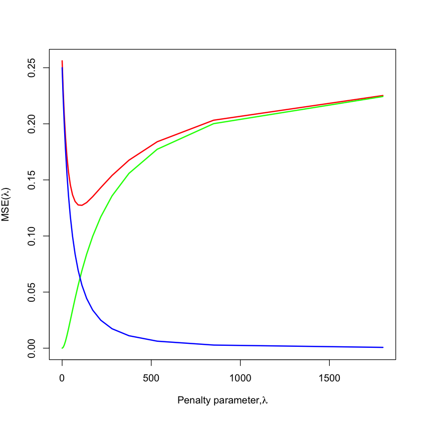
\(\text{Bias}^2\)
\(\text{Variance}\)
\(\text{E[MSE]}\)
How much to shrink?#
In our one-sample example,
Differentiating and solving:
In practice we might hope to estimate MSE with cross-validation.**
plot(alpha, mse, type='l', lwd=2, col='red', ylim=c(0, max(mse)),
     xlab=expression(paste('Shrinkage parameter ', alpha)),
     ylab=expression(paste('MSE(', alpha, ')')))
abline(v=mu^2/(mu^2+sigma^2/nsample), col='blue', lty=2)
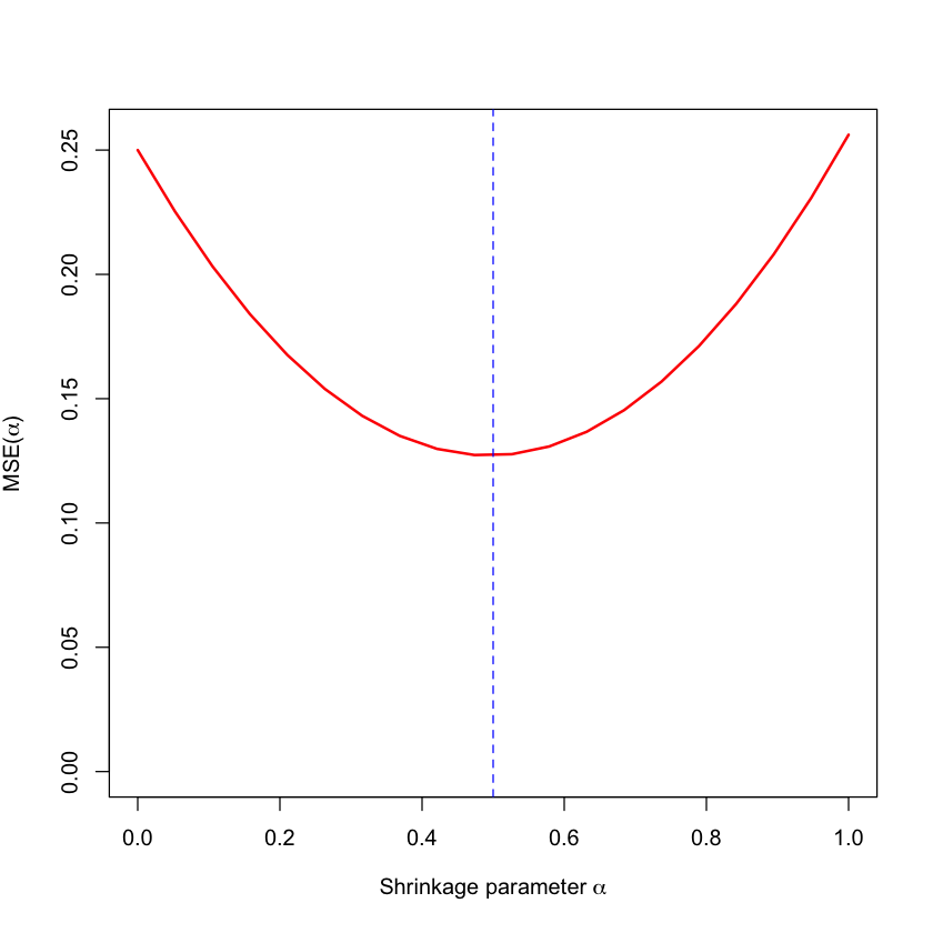
Let’s see how our theoretical choice matches the MSE on our 100 sample.
Penalties & Priors#
Minimizing \(\sum_{i=1}^n (Y_i - \mu)^2 + \lambda \cdot \mu^2\) is similar to computing “MLE” of \(\mu\) if the likelihood was proportional to
If \(\lambda=m\), an integer, then \(\widehat{\mu}_{\lambda}\) is the sample mean of \((Y_1, \dots, Y_n,0 ,\dots, 0) \in \mathbb{R}^{n+m}\).
This is equivalent to adding some data with \(Y=0\) (and some rows to \(X\)).
To a Bayesian, this extra data is a prior distribution and we are computing the so-called MAP or posterior mode.
AIC as penalized regression#
Model selection with \(C_p\) (or AIC with \(\sigma^2\) assumed known) is a version of penalized regression.
The best subsets version of AIC (which is not exactly equivalent to step)
where
is called the \(\ell_0\) norm.
The \(\ell_0\) penalty can be thought of as a measure of complexity of the model. Most penalties are similar versions of complexity.
Ridge regression#
Assume that columns \((X_j)_{1 \leq j \leq p}\) have zero mean, and SD 1 and \(Y\) has zero mean.
This is called the standardized model.
The ridge estimator is
Corresponds (through Lagrange multiplier) to a quadratic constraint on \({\beta_{}}\)’s.
This is the natural generalization of the penalized version of our shrinkage estimator.
Solving the normal equations#
Math aside#
Normal equations
- \[ \implies - \frac{1}{n}(Y - X{\widehat{\beta}_{\lambda}})^T X_l + \lambda {\widehat{\beta}_{l,\lambda}} = 0, \qquad 1 \leq l \leq p\]
In matrix form
Or
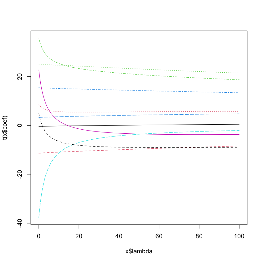
Ridge regression in R#
library(lars)
data(diabetes)
library(MASS)
diabetes.ridge = lm.ridge(diabetes$y ~ diabetes$x,
                          lambda=seq(0, 100, 0.5))
plot(diabetes.ridge, lwd=3)
Loaded lars 1.3
Choosing \(\lambda\)#
If we knew \(E[MSE_{\lambda}]\) as a function of \(\lambda\) then we would simply choose the \(\lambda\) that minimizes it.
To do this, we need to estimate it.
A popular method is cross-validation as a function of \(\lambda\). Breaks the data up into smaller groups and uses part of the data to predict the rest.
We saw this in diagnostics (Cook’s distance measured the fit with and without each point in the data set) and model selection.
\(K\)-fold cross-validation for penalized model#
Fix a model (i.e. fix \(\lambda\)). Break data set into \(K\) approximately equal sized groups \((G_1, \dots, G_K)\).
for (i in 1:K) {
   - Use all groups except `G_i` to fit model, predict outcome in group `G_i` based on this model as `Yhat_i`
   - Estimate `CV = sum([sum((Y[G_i]-Yhat_i)^2) for i in 1:K])/n`
}
CV = function(Z, alpha, K=5) {
    cve = numeric(K)
    n = length(Z)
    for (i in 1:K) {
        g = seq(as.integer((i-1)*n/K)+1,as.integer((i*n/K)))
        mu.hat = mean(Z[-g]) * alpha
        cve[i] = sum((Z[g]-mu.hat)^2)
    }
    return(c(sum(cve) / n, sd(cve) / sqrt(n)))
}
alpha = seq(0.0,1,length=20)
mse = numeric(length(alpha))
avg.cv = numeric(length(alpha))
for (i in 1:ntrial) {
     Z = rnorm(nsample) * sigma + mu
     for (j in 1:length(alpha)) {
         current_cv = CV(Z, alpha[j])
         avg.cv[j] = avg.cv[j] + current_cv[1]
     }
}
avg.cv = avg.cv / ntrial
plot(alpha, avg.cv, type='l', lwd=2, col='green',
     xlab='Shrinkage parameter, alpha', ylab='Average CV(alpha)')
abline(v=mu^2/(mu^2+sigma^2/nsample), col='blue', lty=2)
abline(v=min(alpha[avg.cv == min(avg.cv)]), col='red', lty=2)
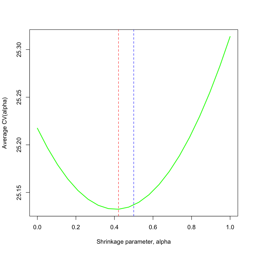
Let’s see how the parameter chosen by 5-fold CV compares to our theoretical choice.
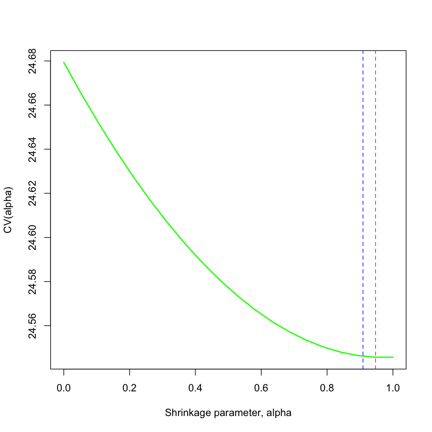
The curve above shows what would happen if we could repeat this and average over many samples. In reality, we only get one sample.
cv = numeric(length(alpha))
cv.sd = numeric(length(alpha))
Z = rnorm(nsample) * sigma + mu
for (j in 1:length(alpha)) {
    current_cv = CV(Z, alpha[j])
    cv[j] = current_cv[1]
    cv.sd[j] = current_cv[2]
}
cv = numeric(length(alpha))
cv.sd = numeric(length(alpha))
nsample = 1000
Z = rnorm(nsample) * sigma + mu
for (j in 1:length(alpha)) {
    current_cv = CV(Z, alpha[j])
    cv[j] = current_cv[1]
    cv.sd[j] = current_cv[2]
}
plot(alpha, cv, type='l', lwd=2, col='green',
    xlab='Shrinkage parameter, alpha', ylab='CV(alpha)', xlim=c(0,1))
 abline(v=mu^2/(mu^2+sigma^2/nsample), col='blue', lty=2)
 abline(v=min(alpha[cv == min(cv)]), col='red', lty=2)
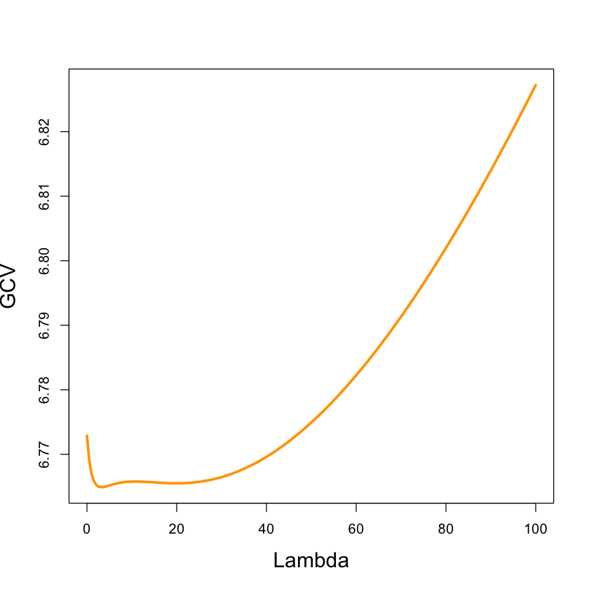
Ridge regression#
par(cex.lab=1.5)
plot(diabetes.ridge$lambda, diabetes.ridge$GCV, xlab='Lambda',
     ylab='GCV', type='l', lwd=3, col='orange')
select(diabetes.ridge)
modified HKB estimator is 5.462251
modified L-W estimator is 7.641667
smallest value of GCV  at 3
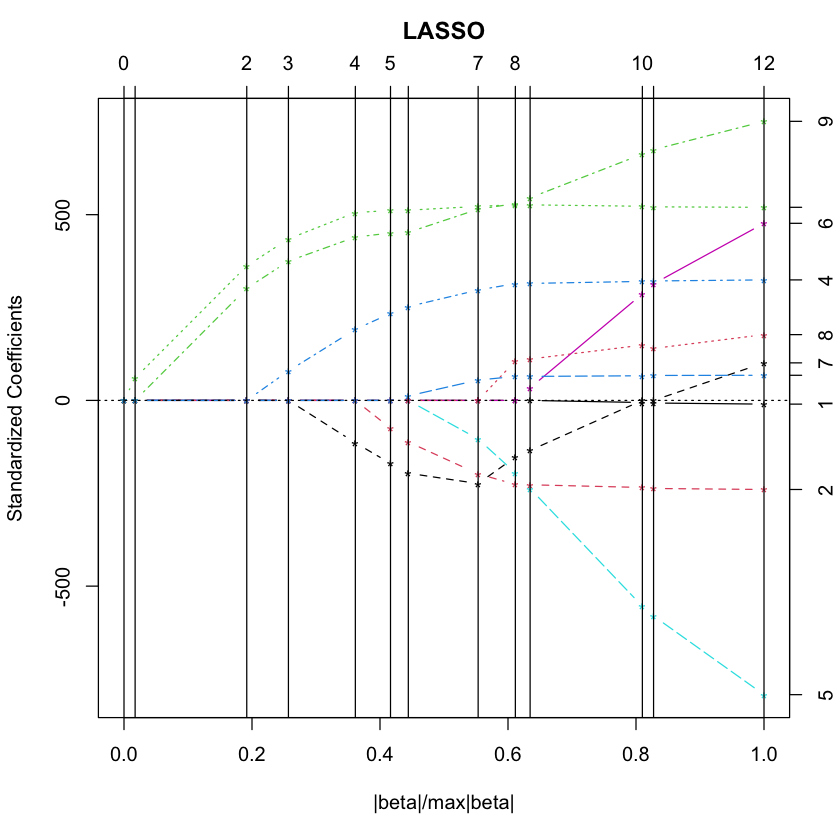
LASSO#
Another popular penalized regression technique. (Again, we standardize)
The LASSO estimate is
Above we defined
is the \(\ell_1\) norm.
Corresponds (through Lagrange multiplier) to an \(\ell_1\) constraint on \({\beta_{}}\)’s.
LASSO#
In theory and practice, it works well when many \({\beta_{j}}\)’s are 0 and gives “sparse” solutions unlike ridge.
It is a (computable) approximation to the best subsets AIC model.
It is computable because the minimization problem is a convex problem.
LASSO#
library(lars)
data(diabetes)
diabetes.lasso = lars(diabetes$x, diabetes$y, type='lasso')
plot(diabetes.lasso)
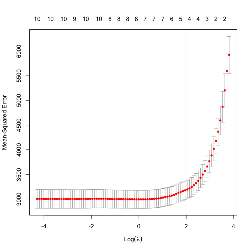
Cross-validation for the LASSO#
The lars package has a built in function to estimate CV.
par(cex.lab=1.5)
cv.lars(diabetes$x, diabetes$y, K=10, type='lasso')

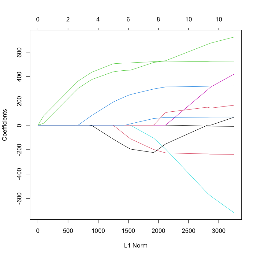
glmnet#
library(glmnet)
G = glmnet(diabetes$x, diabetes$y)
plot(G)
Loading required package: Matrix
Loaded glmnet 4.1-8
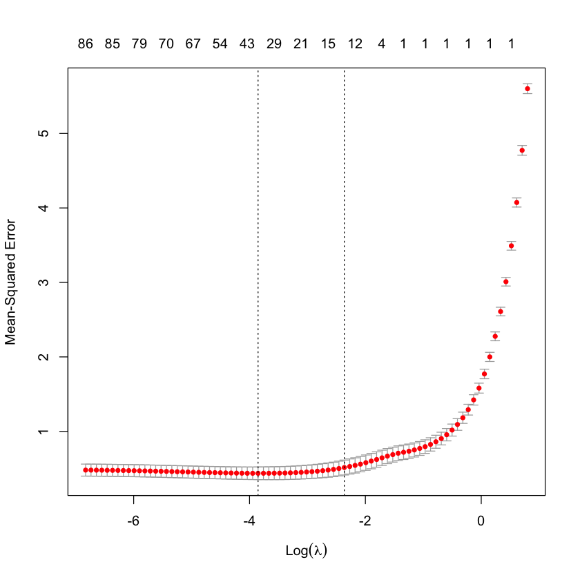
plot(cv.glmnet(diabetes$x, diabetes$y))
cv.glmnet(diabetes$x, diabetes$y)$lambda.1se
HIV example#
Load the data#
url_X = 'https://raw.githubusercontent.com/StanfordStatistics/stats191-data/main/NRTI_X.csv'
url_Y = 'https://raw.githubusercontent.com/StanfordStatistics/stats191-data/main/NRTI_Y.txt'
X_HIV = read.table(url_X, header=FALSE, sep=',')
Y_HIV = read.table(url_Y, header=FALSE, sep=',')
Y_HIV = as.matrix(Y_HIV)[,1]
X_HIV = as.matrix(X_HIV)
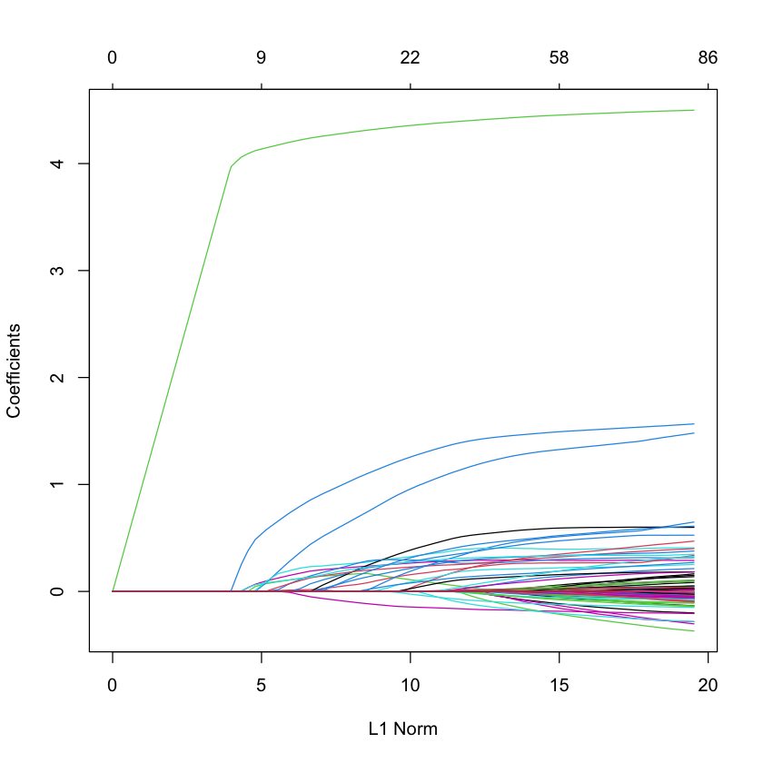
Plot the solution path#
library(glmnet)
G = glmnet(X_HIV, Y_HIV)
plot(G)
CV = cv.glmnet(X_HIV, Y_HIV)
plot(CV)