Course Introduction#
Download#
Course overview#
Review++ (e.g. STATS60 and a little more)
Beyond \(t\)-tests
Multiple group: ANOVA
Simple linear regression
Multiple linear regression
Model diagnostics
Model selection
Logistic regression
…
What is course about?#
It is a course on applied statistics.
Hands-on: we use R, an open-source statistics software environment.
Course notes will be available as jupyter notebooks.
We will start out with a review of introductory statistics to see
Rin action.Main topic is (linear) regression models: these are the bread and butter of applied statistics.
What is a regression model?#
A regression model is a model of the relationships between some covariates (predictors) and an outcome.
Specifically, regression is a model of the average outcome given or having fixed the covariates.
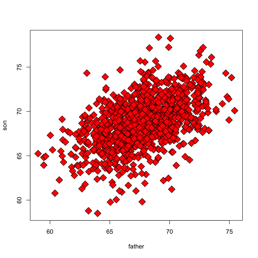
Heights of fathers and sons#
We will consider the of fathers and sons collected by Karl Pearson in the late 19th century. Perhaps the first regression model!
One of our goals is to understand height of the son,
S, knowing the height of the father,F.A mathematical model might look like
\[ S = g(F) + \varepsilon\]Above \(g\) gives the average height of the son of a father of height
Fand \(\varepsilon\) is error: not every son whose fathers have the same height themselves have the same height.A statistical question: is there any relationship between covariates and outcomes – is \(g\) just a constant?
require(UsingR)
heights = UsingR::father.son
father = heights$fheight
son = heights$sheight
Loading required package: UsingR
Loading required package: MASS
Loading required package: HistData
Loading required package: Hmisc
Attaching package: ‘Hmisc’
The following objects are masked from ‘package:base’:

    format.pval, units
plot(father, son, pch = 23, bg = "red", cex = 2)
Line of best fit#
plot(father, son, pch=23, bg="red", cex=2)
height.lm = lm(son ~ father)
abline(height.lm, lwd=4, col="black", lty=2)
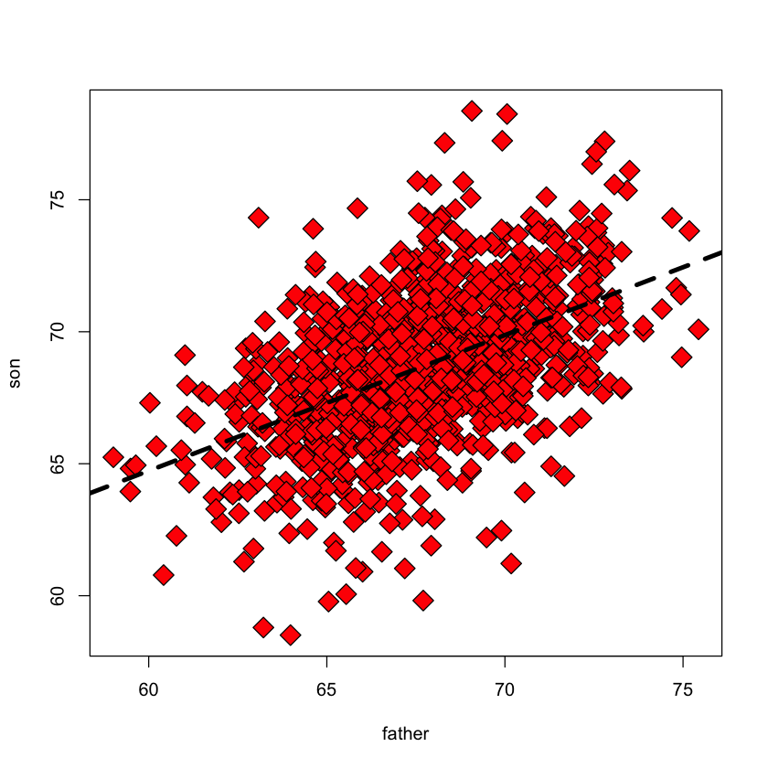
Linear regression model#
How do we find this line? With a model.
We might model the data as
This model is linear in \((\beta_0, \beta_1)\), the intercept and the coefficient of
F(the father’s height), it is a simple linear regression model.
Another model#
Also linear (in \((\beta_0, \beta_1, \beta_2)\), the coefficients of \(1, F, F^2\)).
Which model is better? We will need a tool to compare models… more to come later.
Our example here was rather simple: we only had one independent variable:
F.
Multiple linear regression: brain size in mammals#
brains = read.csv('https://raw.githubusercontent.com/StanfordStatistics/stats191-data/main/Sleuth3/brains.csv', header=TRUE)
rownames(brains) = brains$Species
brains = brains[,2:5]
head(brains)
| Brain | Body | Gestation | Litter | |
|---|---|---|---|---|
| <dbl> | <dbl> | <int> | <dbl> | |
| Aardvark | 9.6 | 2.20 | 31 | 5.0 |
| Acouchis | 9.9 | 0.78 | 98 | 1.2 |
| African elephant | 4480.0 | 2800.00 | 655 | 1.0 |
| Agoutis | 20.3 | 2.80 | 104 | 1.3 |
| Axis deer | 219.0 | 89.00 | 218 | 1.0 |
| Badger | 53.0 | 6.00 | 60 | 2.2 |
Features and response#
Response in brains#
Brain: average brain weight (in grams)
Features in brains#
Body: average body weight (in kilograms)Gestation: gestation period (in days)Litter: average litter size
Graphical exploration#
pairs(brains)

Building a model#
Some of the main goals of this course:
Build a statistical model describing the effect of
GestationonBrain.This model should recognize that other variables also affect
Brain.What sort of statistical conclusions can we make based on our model?
Is the model we choose adequate describe this dataset?
Are there other (simpler, more complicated) better models?