Simple Linear Regression Assumptions#
Download#
Outline#
Goodness of fit of regression: analysis of variance.
\(F\)-statistics.
Residuals.
Diagnostic plots.
 {height=600 fig-align=”center”}
Figure depicts the statistical model for regression:#
First we start with \(X\), then compute the mean \(\beta_0 + \beta_1 X\) then add error \(\epsilon\) yielding
Geometry of least squares#
Full model#
This is the model
Its fitted values are
Reduced model#
This is the model
Its fitted values are
Regression sum of squares#
The closer \(\hat{Y}\) is to the \({1}\) axis, the less “variation” there is along the \(X\) axis.
This closeness can be measured by the length of the vector \(\hat{Y}-\bar{Y} \cdot 1\).
Its length is
An important right triangle#
 {height=300 fig-align=”center”}
Sides of the triangle: SSR, SSE
Hypotenuse: SST
Degrees of freedom in the right triangle#
 {height=300 fig-align=”center”}
Sides of the triangle: SSR has 1 d.f., SSE has n-2 d.f.
Hypotenuse: SST has n-1 d.f.
Mean squares#
Each sum of squares gets an extra bit of information associated to them, called their degrees of freedom.
Roughly speaking, the degrees of freedom can be determined by dimension counting.
Computing degrees of freedom#
The \(SSE\) has \(n-2\) degrees of freedom because it is the squared length of a vector that lies in \(n-2\) dimensions. To see this, note that it is perpendicular to the 2-dimensional plane formed by the \(X\) axis and the \(1\) axis.
The \(SST\) has \(n-1\) degrees of freedom because it is the squared length of a vector that lies in \(n-1\) dimensions. In this case, this vector is perpendicular to the \(1\) axis.
The \(SSR\) has 1 degree of freedom because it is the squared length of a vector that lies in the 2-dimensional plane but is perpendicular to the \(1\) axis.
A different visualization#
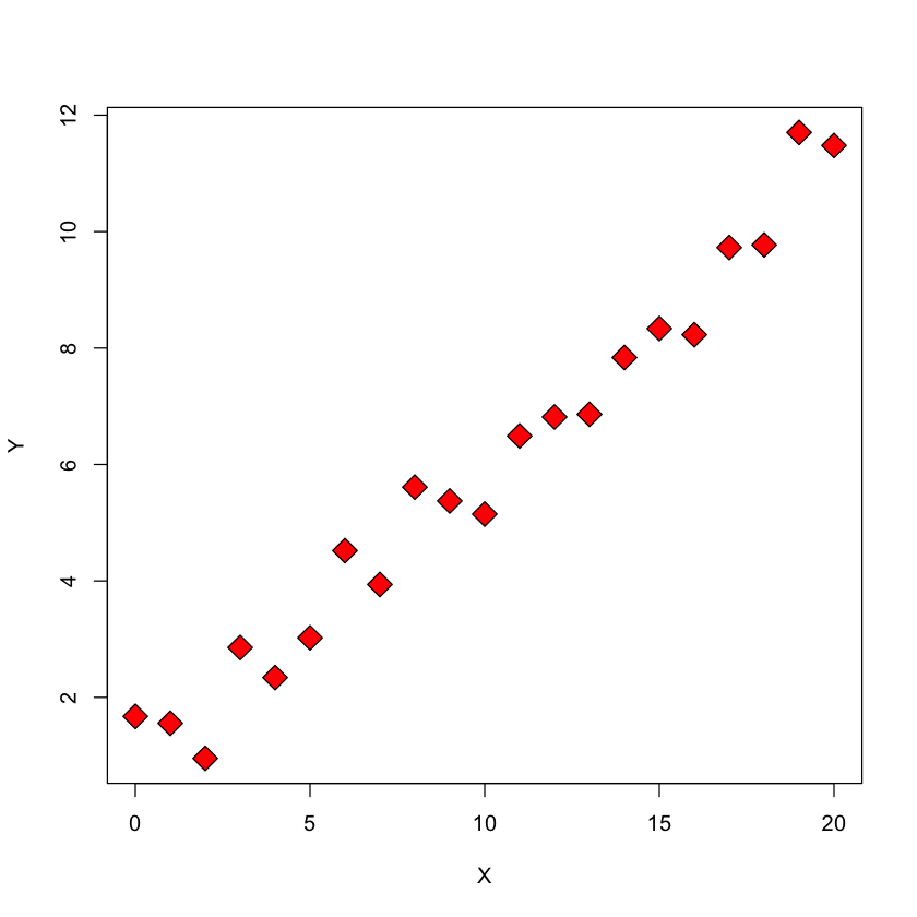
These sums of squares can be visualized by other means as well. We will illustrate with a synthetic dataset.
X = seq(0, 20, length = 21)
Y = 0.5 * X + 1 + rnorm(21)
plot(X,Y, pch=23, bg='red', cex=2)
SST: total sum of squares#
plot(X, Y, pch = 23, bg = "red", main='Total sum of squares', cex=2)
abline(h = mean(Y), col = "yellow", lwd = 2)
for (i in 1:21) {
      points(X[i], mean(Y), pch = 23, bg = "yellow")
      lines(c(X[i], X[i]), c(Y[i], mean(Y)))
}

Description#
This figure depicts the **total sum of squares, \(SST\) ** – the sum of the squared differences between the Y values and the sample mean of the Y values.
SSE: error sum of squares#
plot(X, Y, pch = 23, bg = "red", main="Error sum of squares", cex=2)
Y.lm = lm(Y ~ X)
Yhat = predict(Y.lm)
abline(Y.lm, col = "green", lwd = 2)
for (i in 1:21) {
    points(X[i], Yhat[i], pch = 23, bg = "green")
    lines(c(X[i], X[i]), c(Y[i], Yhat[i]))
}
abline(h = mean(Y), col = "yellow", lwd = 2)
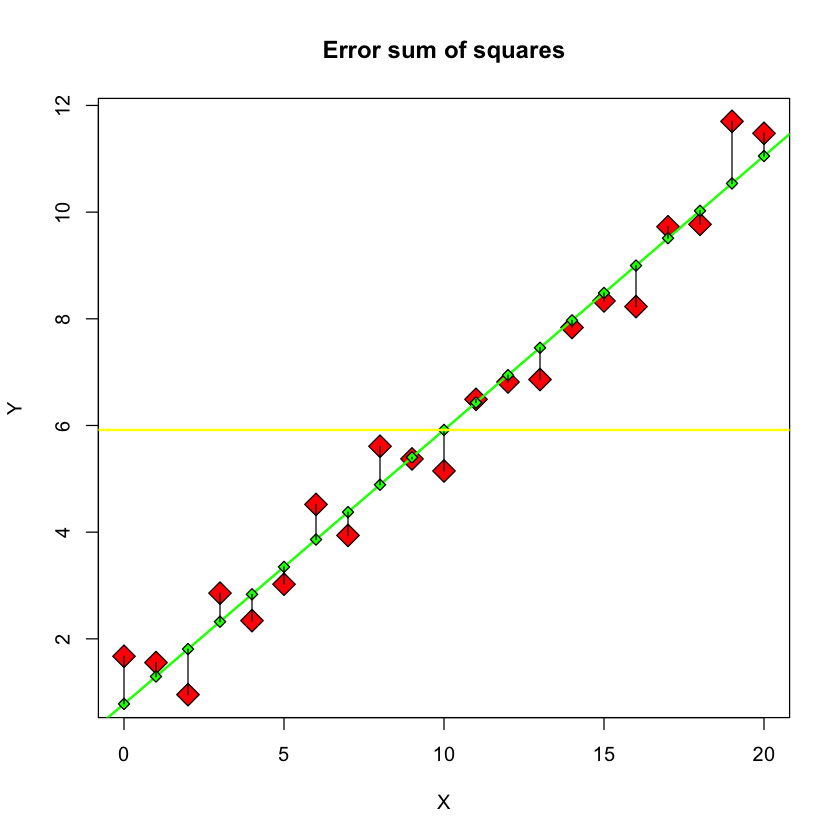
Description#
This figure depicts the **error sum of squares, \(SSE\) ** - the sum of the squared differences between the \(Y\) values and the \(\hat{Y}\) values, i.e. the fitted values of the regression model.
SSR: regression sum of squares#
plot(X, Y, pch = 23, bg = "red", main="Regression sum of squares", cex=2)
abline(Y.lm, col = "green", lwd = 2)
abline(h = mean(Y), col = "yellow", lwd = 2)
for (i in 1:21) {
     points(X[i], Yhat[i], pch = 23, bg = "green")
     points(X[i], mean(Y), pch = 23, bg = "yellow")
     lines(c(X[i], X[i]), c(mean(Y), Yhat[i]))
}

Description#
This figure depicts the **regression sum of squares, \(SSR\) ** - the sum of the squared differences between the \(\hat{Y}\) values and the sample mean of the \(Y\) values.
Definition of \(R^2\)#
As noted above, if the regression model fits very well, then \(SSR\) will be large relative to \(SST\). The \(R^2\) score is just the ratio of these sums of squares.
Let’s verify this on the big_bang data.
url = 'https://raw.githubusercontent.com/StanfordStatistics/stats191-data/main/Sleuth3/big_bang.csv'
big_bang = read.table(url, sep=',', header=TRUE)
big_bang.lm = lm(Distance ~ Velocity, data=big_bang)
Let’s verify our claim \(SST=SSE+SSR\):
SSE = sum(resid(big_bang.lm)^2)
SST = with(big_bang, sum((Distance - mean(Distance))^2))
SSR = with(big_bang, sum((mean(Distance) - predict(big_bang.lm))^2))
c(SST, SSE + SSR) # these values are the same
- 9.5906625
- 9.5906625
\(R^2\) and correlation#
Finally, \(R=\sqrt{R^2}\) is called the (absolute) correlation coefficient because it is equal to the absolute value of sample correlation coefficient of \(X\) and \(Y\).
with(big_bang, cor(Velocity, Distance)^2)
\(F\)-statistics#
After a \(t\)-statistic, the next most commonly encountered statistic is a \(\chi^2\) statistic, or its closely related cousin, the \(F\) statistic.
A \(\chi^2_k\) random variable is the distribution of the squared length of a centered normal vector in \(k\) dimensions (proper definition needs slightly more detail).
Sums of squares are squared lengths!
\(F\) statistic for simple linear regression#
Defined as
Can be thought of as a ratio of a difference in sums of squares normalized by our “best estimate” of variance .
\(F\) statistics and \(R^2\)#
The \(R^2\) is also closely related to the \(F\) statistic reported as the goodness of fit in summary of lm.
F = (SSR / 1) / (SSE / big_bang.lm$df)
F
summary(big_bang.lm)$fstatistic
anova(big_bang.lm)
- value
- 36.2891901954741
- numdf
- 1
- dendf
- 22
| Df | Sum Sq | Mean Sq | F value | Pr(>F) | |
|---|---|---|---|---|---|
| <int> | <dbl> | <dbl> | <dbl> | <dbl> | |
| Velocity | 1 | 5.970873 | 5.9708734 | 36.28919 | 4.607681e-06 |
| Residuals | 22 | 3.619789 | 0.1645359 | NA | NA |
Simple manipulations yield
22*0.6226 / (1 - 0.6226)
\(F\) test under \(H_0\)#
Under \(H_0:\beta_1=0\),
because
and from our “right triangle”, these vectors are orthogonal.
The null hypothesis \(H_0:\beta_1=0\) implies that \(SSR \sim \chi^2_1 \cdot \sigma^2\).
\(F\)-statistics and mean squares#
An \(F\)-statistic is a ratio of mean squares: it has a numerator, \(N\), and a denominator, \(D\) that are independent.
Let
and define
We say \(F\) has an \(F\) distribution with parameters \(df_{{\rm num}}, df_{{\rm den}}\) and write \(F \sim F_{df_{{\rm num}}, df_{{\rm den}}}\)
Takeaway#
\(F\) statistics are computed to test some \(H_0\).
When that \(H_0\) is true, the \(F\) statistic has this \(F\) distribution (with appropriate degrees of freedom).
Relation between \(F\) and \(t\) statistics.#
If \(T \sim t_{\nu}\), then
\[ T^2 \sim \frac{N(0,1)^2}{\chi^2_{\nu}/\nu} \sim \frac{\chi^2_1/1}{\chi^2_{\nu}/\nu}.\]In other words, the square of a \(t\)-statistic is an \(F\)-statistic. Because it is always positive, an \(F\)-statistic has no direction associated with it.
In fact
\[ F = \frac{MSR}{MSE} = \frac{\widehat{\beta}_1^2}{SE(\widehat{\beta}_1)^2}.\]
Verifying \(F\)-statistic calculation#
Let’s check this in our example.
summary(big_bang.lm)$fstatistic
- value
- 36.2891901954741
- numdf
- 1
- dendf
- 22
The \(t\) statistic for education is the \(t\)-statistic for the parameter \(\beta_1\) under \(H_0:\beta_1=0\). Its value is 6.024 above. If we square it, we should get about the same as the F-statistic.
6.024**2
Interpretation of an \(F\)-statistic#
In regression, the numerator is usually a difference in goodness of fit of two (nested) models.
The denominator is \(\hat{\sigma}^2\) – an estimate of \(\sigma^2\).
In our example today: the bigger model is the simple linear regression model, the smaller is the model with constant mean (one sample model).
If the \(F\) is large, it says that the bigger model explains a lot more variability in \(Y\) (relative to \(\sigma^2\)) than the smaller one.
Analysis of variance#
The \(F\)-statistic has the form
Right triangle with full and reduced model: sum of squares#
 {height=300 fig-align=”center”}
Sides of the triangle: \(SSE_R-SSE_F\), \(SSE_F\)
Hypotenuse: \(SSE_R\)
Right triangle with full and reduced model: degrees of freedom#
 {height=300 fig-align=”center”}
Sides of the triangle: \(df_R-df_F\), \(df_F\)
Hypotenuse: \(df_R\)
The \(F\)-statistic for simple linear regression revisited#
The null hypothesis is
The usual \(\alpha\) rejection rule would be to reject \(H_0\) if the \(F_{\text{obs}}\) the observed \(F\) statistic is greater than \(F_{1,n-2,1-\alpha}\).
In our case, the observed \(F\) was 36.3, \(n-2=22\) and the appropriate 5% threshold is computed below to be 4.30. Therefore, we strongly reject \(H_0\).
qf(0.95, 1, 22)
Case study B: breakdown time for insulating fluid#
url = 'https://raw.githubusercontent.com/StanfordStatistics/stats191-data/main/Sleuth3/fluid_breakdown.csv'
breakdown = read.table(url, sep=',', header=TRUE)
with(breakdown, plot(Voltage, Time))

breakdown.lm = lm(Time ~ Voltage, data=breakdown)
summary(breakdown.lm)$coef
summary(breakdown.lm)$fstatistic
| Estimate | Std. Error | t value | Pr(>|t|) | |
|---|---|---|---|---|
| (Intercept) | 1886.16946 | 364.48122 | 5.174943 | 1.886969e-06 |
| Voltage | -53.95492 | 10.95264 | -4.926203 | 4.965655e-06 |
- value
- 24.267474478293
- numdf
- 1
- dendf
- 74
A designed experiment to estimate average breakdown time under different voltages.
Another model#
full.lm = lm(Time ~ factor(Voltage), data=breakdown)
summary(full.lm)$coef
summary(full.lm)$fstatistic
| Estimate | Std. Error | t value | Pr(>|t|) | |
|---|---|---|---|---|
| (Intercept) | 1303.0033 | 132.3377 | 9.846051 | 8.809748e-15 |
| factor(Voltage)28 | -946.7833 | 167.3954 | -5.655971 | 3.242824e-07 |
| factor(Voltage)30 | -1227.2215 | 149.2970 | -8.220001 | 7.914303e-12 |
| factor(Voltage)32 | -1261.8407 | 144.9686 | -8.704232 | 1.031985e-12 |
| factor(Voltage)34 | -1288.6444 | 142.4026 | -9.049303 | 2.427522e-13 |
| factor(Voltage)36 | -1298.3973 | 144.9686 | -8.956402 | 3.582214e-13 |
| factor(Voltage)38 | -1302.0871 | 155.1797 | -8.390836 | 3.855139e-12 |
- value
- 16.1227405670227
- numdf
- 6
- dendf
- 69
There were only 7 distinct values of
Voltage: can be treated as a category (i.e.factor)
A different reduced & full model#
anova(breakdown.lm, full.lm)
| Res.Df | RSS | Df | Sum of Sq | F | Pr(>F) | |
|---|---|---|---|---|---|---|
| <dbl> | <dbl> | <dbl> | <dbl> | <dbl> | <dbl> | |
| 1 | 74 | 6557345 | NA | NA | NA | NA |
| 2 | 69 | 3625244 | 5 | 2932102 | 11.16146 | 6.674496e-08 |
Our “right triangle” again (only degrees of freedom this time):#
 {height=300 fig-align=”center”}
Sides of the triangle: \(df_R-df_F=5\), \(df_F=69\)
Hypotenuse: \(df_R=74\)
Diagnostics for simple linear regression#
What can go wrong?#
Using a linear regression function can be wrong: maybe regression function should be quadratic.
We assumed independent Gaussian errors with the same variance. This may be incorrect.
The errors may not be normally distributed.
The errors may not be independent.
The errors may not have the same variance.
Detecting problems is more art then science, i.e. we cannot test for all possible problems in a regression model.
Inspecting residuals#
The basic idea of most diagnostic measures is the following:
If the model is correct then residuals \(e_i = Y_i -\widehat{Y}_i, 1 \leq i \leq n\) should look like a sample of (not quite independent) \(N(0, \sigma^2)\) random variables.
A poorly fitting model#
y = anscombe$y2 + rnorm(length(anscombe$y2)) * 0.45
x = anscombe$x2
plot(x, y, pch = 23, bg = "orange", cex = 2, ylab = "Y",
     xlab = "X")
simple.lm = lm(y ~ x)
abline(simple.lm, lwd = 2, col = "red", lty = 2)
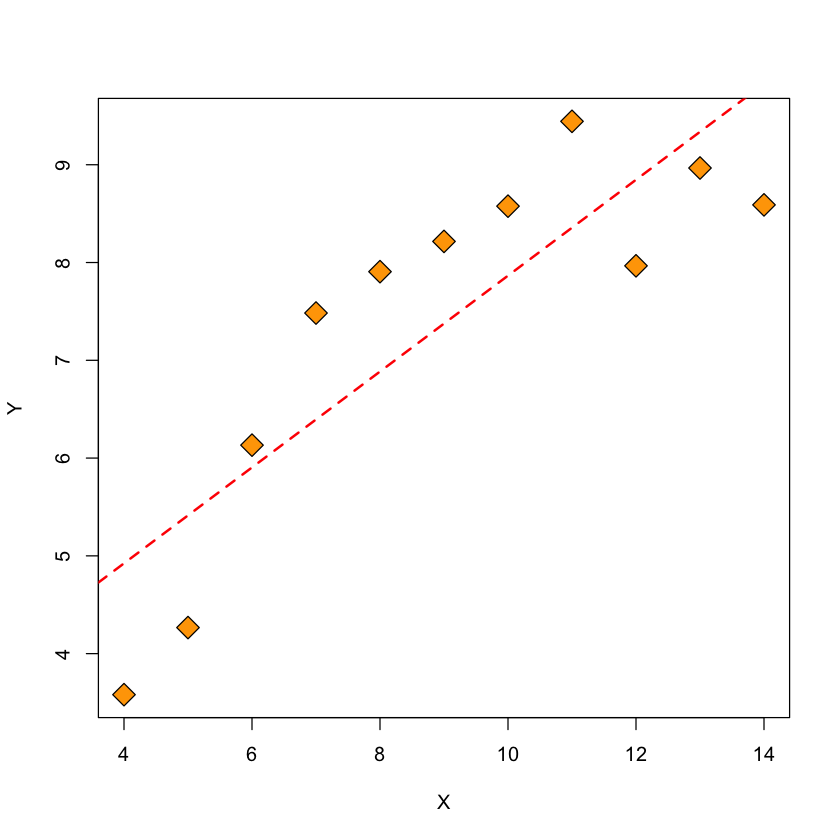
Figure: \(Y\) vs. \(X\) and fitted regression line#
Residuals for Anscombe’s data#
plot(x, resid(simple.lm), ylab = "Residual", xlab = "X", pch = 23,
        bg = "orange", cex = 2)
abline(h = 0, lwd = 2, col = "red", lty = 2)
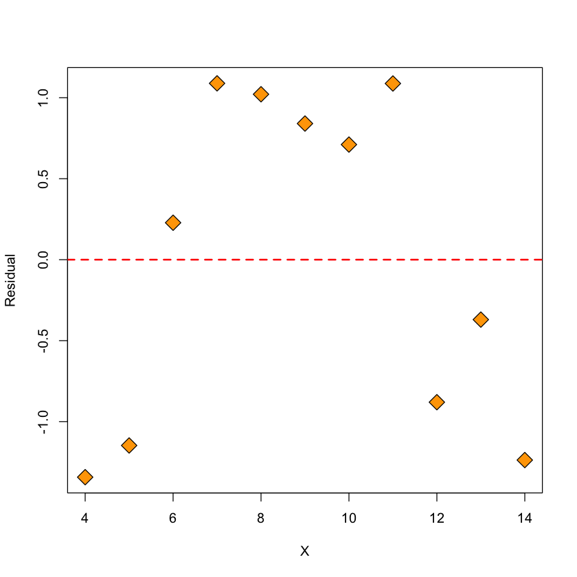
Figure: residuals vs. \(X\)#
Quadratic model#
Let’s add a quadratic term to our model (a multiple linear regression model).
quadratic.lm = lm(Y ~ poly(X, 2))
quadratic.lm = lm(y ~ poly(x, 2))
Xsort = sort(x)
plot(x, y, pch = 23, bg = "orange", cex = 2, ylab = "Y",
     xlab = "X")
lines(Xsort, predict(quadratic.lm, list(x = Xsort)), col = "red", lty = 2,
      lwd = 2)
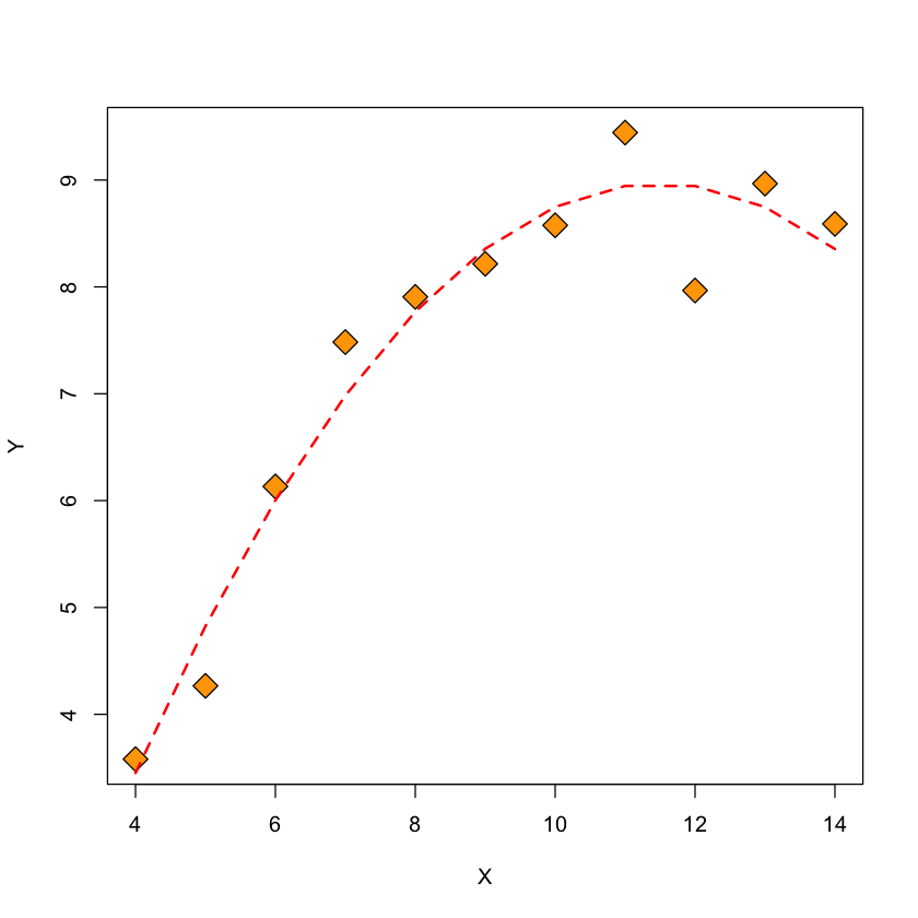
Figure: \(Y\) and fitted quadratic model vs. \(X\)#
Inspecting residuals of quadratic model#
The residuals of the quadratic model have no apparent pattern in them, suggesting this is a better fit than the simple linear regression model.
plot(x, resid(quadratic.lm), ylab = "Residual", xlab = "X", pch = 23,
        bg = "orange", cex = 2)
abline(h = 0, lwd = 2, col = "red", lty = 2)

Figure: residuals of quadratic model vs. \(X\)#
Assessing normality of errors: QQ-plot for linear model#
qqnorm(resid(simple.lm), pch = 23, bg = "orange", cex = 2)
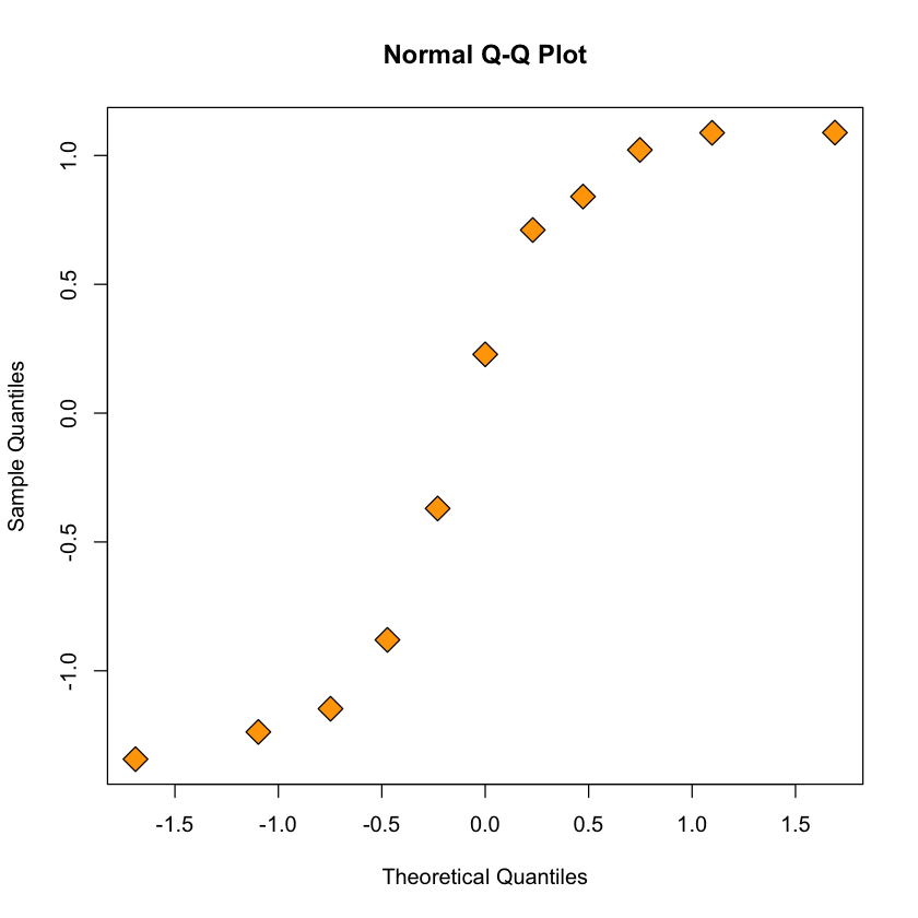
Figure: quantiles of poorly fitting model’s residuals vs. expected Gaussian quantiles#
QQ-plot for quadratic model#
qqnorm(resid(quadratic.lm), pch = 23, bg = "orange", cex = 2)
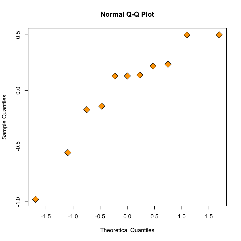
Figure: quantiles of quadratic model’s residuals vs. expected Gaussian quantiles#
qqnormdoes not seem vastly different \(\implies\) several diagnostic tools can be useful in assessing a model.
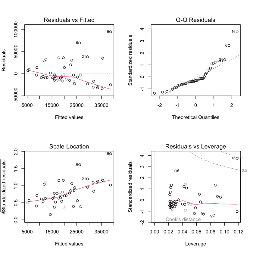
Default plots in R#
par(mfrow=c(2,2)) # this makes 2x2 grid of plots
plot(simple.lm)
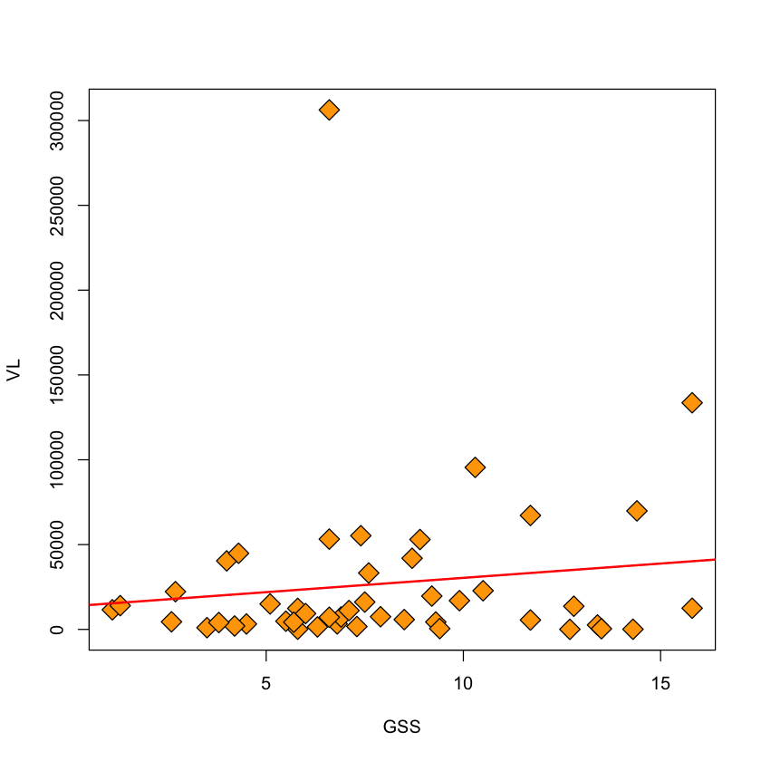
Assessing constant variance assumption#
url = 'https://raw.githubusercontent.com/StanfordStatistics/stats191-data/main/HIV.VL.table'
viral.load = read.table(url, header=TRUE)

with(viral.load, plot(GSS, VL, pch=23, bg='orange', cex=2))
viral.lm = lm(VL ~ GSS, data=viral.load)
abline(viral.lm, col='red', lwd=2)
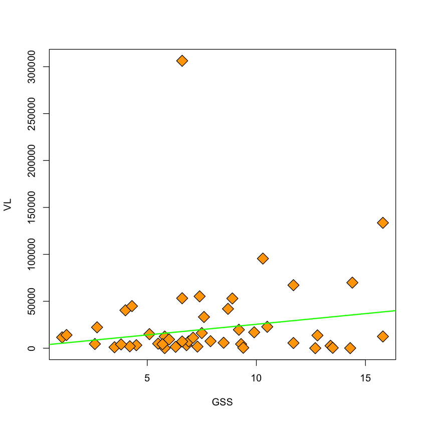
Removing an outlier#
viral.load$keep = (viral.load$VL < 200000)
with(viral.load, plot(GSS, VL, pch=23, bg='orange', cex=2))
viral.lm.good = lm(VL ~ GSS, subset=keep, data=viral.load)
abline(viral.lm.good, col='green', lwd=2)
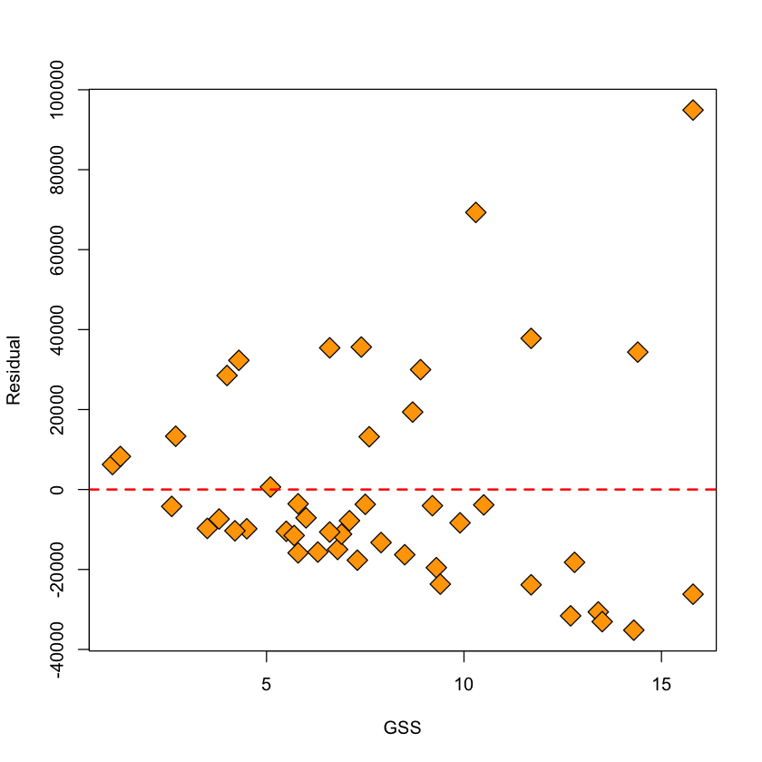
Heteroscedastic errors#
When we plot the residuals against the fitted values for this model (even with the outlier removed) we see that the variance clearly depends on \(GSS\). They also do not seem symmetric around 0 so perhaps the Gaussian model is not appropriate.
with(viral.load,
     plot(GSS[keep], resid(viral.lm.good), pch=23,
          bg='orange', cex=2, xlab='GSS', ylab='Residual'))
abline(h=0, lwd=2, col='red', lty=2)
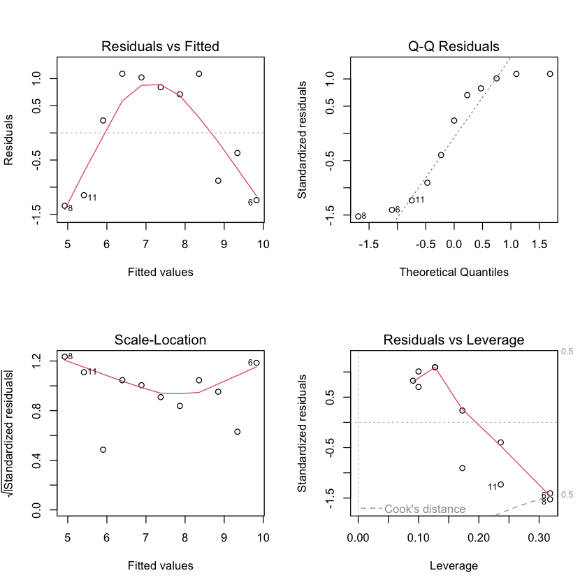
Plots from lm#
We can see some of these plots in
R:
par(mfrow=c(2,2))
plot(viral.lm.good)