Model selection

Download

• Slides

• RStudio: RMarkdown,Quarto

• Jupyter

Outline

• Case studies:

  A. SAT scores by state

  B. Deeper dive into sex discrimination in base salary

• Model selection

• Best subsets

• Stepwise methods

Case study A: State SAT scores

• Predicting average 1982 SAT score by state.

• Features:

  1. Takers (percentage)

  2. Income (parental income of SAT takers)

  3. Years (years of education in key subjects)

  4. Public (percent of takers in public high school)

  5. Expend (state expenditure on high schools per student)

  6. Rank (average percentile of students writing SAT

SAT data

url = 'https://raw.githubusercontent.com/StanfordStatistics/stats191-data/main/Sleuth3/state_SAT.csv'
SAT.df = read.csv(url, sep=',', row.names=1, header=TRUE)
head(SAT.df)

A data.frame: 6 × 7

	SAT	Takers	Income	Years	Public	Expend	Rank
	<int>	<int>	<int>	<dbl>	<dbl>	<dbl>	<dbl>
Iowa	1088	3	326	16.79	87.8	25.60	89.7
SouthDakota	1075	2	264	16.07	86.2	19.95	90.6
NorthDakota	1068	3	317	16.57	88.3	20.62	89.8
Kansas	1045	5	338	16.30	83.9	27.14	86.3
Nebraska	1045	5	293	17.25	83.6	21.05	88.5
Montana	1033	8	263	15.91	93.7	29.48	86.4

Case study B: Sex discrimination in employment

• Same data as earlier, with additional features:

  1. Age (years)

  2. Educ (years)

  3. Exper (months)

  4. Senior (months)

  5. Sal77 (salary in 1977 – used for a different analysis in the book)

Salary data

url = 'https://raw.githubusercontent.com/StanfordStatistics/stats191-data/main/Sleuth3/discrim_employment.csv'
salary = read.table(url, sep=',', header=TRUE)
head(salary)

A data.frame: 6 × 7

	Bsal	Sal77	Sex	Senior	Age	Educ	Exper
	<int>	<int>	<chr>	<int>	<int>	<int>	<dbl>
1	5040	12420	Male	96	329	15	14.0
2	6300	12060	Male	82	357	15	72.0
3	6000	15120	Male	67	315	15	35.5
4	6000	16320	Male	97	354	12	24.0
5	6000	12300	Male	66	351	12	56.0
6	6840	10380	Male	92	374	15	41.5

Model selection

• In a given regression situation, there are often many choices to be made. Recall our usual setup (with intercept)

(28)\[\begin{equation} Y_{n \times 1} = X_{n \times (p+1)} \beta_{(p+1) \times 1} + \epsilon_{n \times 1}. \end{equation}\]

• Any subset \(A \subset \{1, \dots, p\}\) yields a new regression model

(29)\[\begin{equation} {\cal M}(A): Y_{n \times 1} = X[,A] \beta[A] + \epsilon_{n \times 1} \end{equation}\]

Why model selection?

Possible goals in the SAT data

• States with low Takers typically have high Rank

• Beyond this effect, what is important for understanding variability in SAT scores?

• Maybe want a parsimonious model.

General problem & goals

• When we have many predictors (with many possible interactions), it can be difficult to formulate a good model from outside considerations.

• Which main effects do we include?

• Which interactions do we include?

• Model selection procedures try to simplify / automate this task.

General comments

• This is generally an “unsolved” problem in statistics: there are no magic procedures to get you the “best model” or “correct model”.

• Inference after selection is full of pitfalls!

General approach

• To “implement” a model selection procedure, we first need a criterion / score / benchmark to compare two models.

• Given a criterion, we also need a search strategy.

Search strategies

• Exhaustive: With a limited number of predictors, it is possible to search all possible models.

• Sequential: Select a model in a sequence of steps.

Exhaustive search (leaps in R)

Candidate criteria

• \(R^2\): not a good criterion. Always increase with model size \(\implies\) “optimum” is to take the biggest model.

• Adjusted \(R^2\): better. It “penalized” bigger models. Follows principle of parsimony / Occam’s razor.

• Mallow’s \(C_p\) – attempts to estimate a model’s predictive power, i.e. the power to predict a new observation.

Setup for leaps

# you may need to install `leaps` library
# install.packages('leaps', repos='http://cloud.r-project.org')
library(leaps) 

• leaps takes a design matrix as argument: throw away the intercept column or leaps will complain:

SAT.lm = lm(SAT ~ ., SAT.df)
X_SAT = model.matrix(SAT.lm)[,-1]
Y_SAT = SAT.df$SAT

The problem with R^2

SAT.leaps = leaps(X_SAT, Y_SAT, nbest=5, method='r2')
r2_idx = which((SAT.leaps$r2 == max(SAT.leaps$r2)))
best.model.r2 = colnames(X_SAT)[SAT.leaps$which[r2_idx,]]
best.model.r2

1. 'Takers'
2. 'Income'
3. 'Years'
4. 'Public'
5. 'Expend'
6. 'Rank'

---

plot(SAT.leaps$size, 
     SAT.leaps$r2, 
     pch=23, 
     bg='orange', 
     cex=2,
     ylab='R^2',
     xlab='Model size')
points(SAT.leaps$size[r2_idx],
       SAT.leaps$r2[r2_idx],
       pch=24,
       bg='red', 
       cex=3)

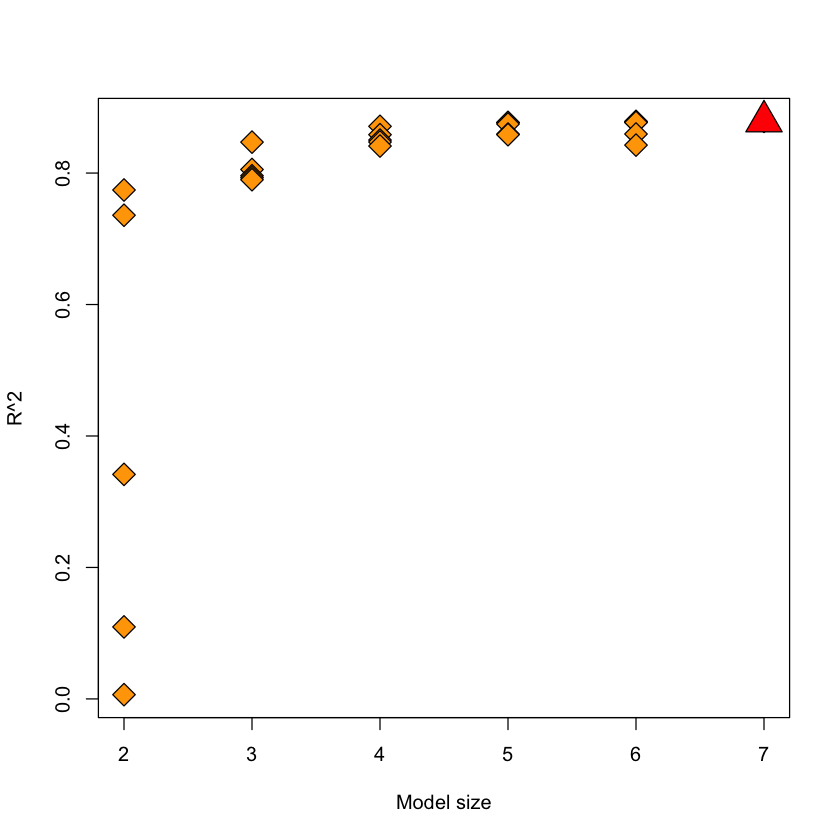
Figure

• Plot of \(R^2\) of a model as a function of the model size.

• The “best” model in terms of \(R^2\) does indeed include all variables.

Adjusted \(R^2\)

• As we add more and more variables to the model – even random ones, \(R^2\) will increase to 1.

• Recall that adjusted \(R^2\) tries to take this into account by replacing sums of squares by mean squares

\[R^2_a = 1 - \frac{SSE/(n-p-1)}{SST/(n-1)} = 1 - \frac{MSE}{MST}.\]

SAT.leaps = leaps(X_SAT, Y_SAT, nbest=5, method='adjr2')
adjr2_idx = which((SAT.leaps$adjr2 == max(SAT.leaps$adjr2)))
best.model.adjr2 = colnames(X_SAT)[SAT.leaps$which[adjr2_idx,]]
best.model.adjr2

1. 'Years'
2. 'Public'
3. 'Expend'
4. 'Rank'

---

plot(SAT.leaps$size, 
     SAT.leaps$adjr2, 
     pch=23, bg='orange', 
     cex=2,
     ylab='Adjusted R^2',
     xlab='Model size')
points(SAT.leaps$size[adjr2_idx],
       SAT.leaps$adjr2[adjr2_idx],
       pch=24, bg='red', cex=3)

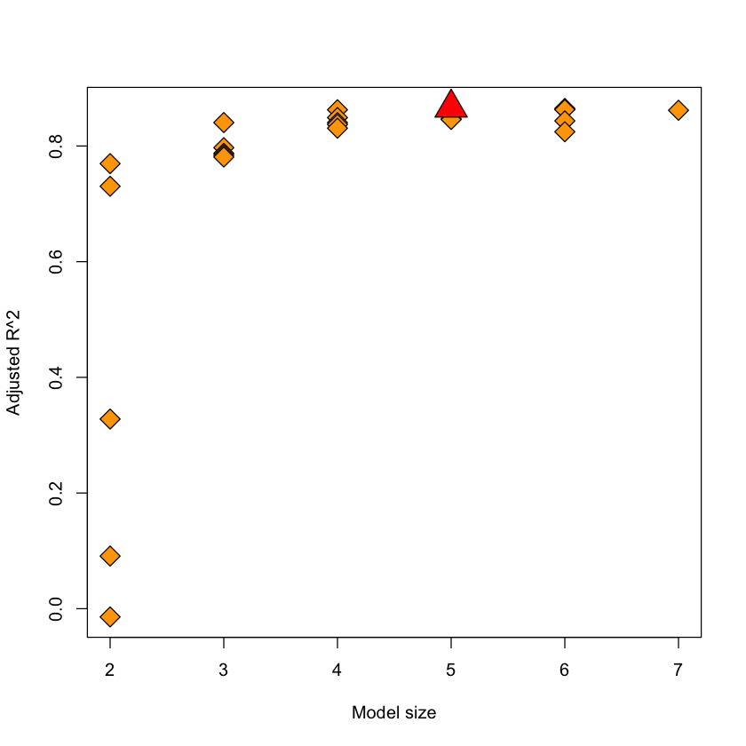
Figure

• Plot of \(R^2_a\) of a model as a function of the model size.

• The “best” model in terms of \(R^2_a\) is not the full model: has size 5 (4 variables plus intercept)

Mallow’s \(C_p\)

Definition:

\[C_p({\cal M}) = \frac{SSE({\cal M})}{\widehat{\sigma}^2} + 2 \cdot p({\cal M}) - n.\]

Notes:

• \(\widehat{\sigma}^2=SSE(F)/df_F\) is the “best” estimate of \(\sigma^2\) we have (use the fullest model), i.e. in the SAT data it uses all 6 main effects.

• \(SSE({\cal M})\) is the \(SSE\) of the model \({\cal M}\).

• \(p({\cal M})\) is the number of predictors in \({\cal M}\).

• This is an estimate of the expected mean-squared error of \(\widehat{Y}({\cal M})\), it takes bias and variance into account.

---

SAT.leaps = leaps(X_SAT, Y_SAT, nbest=3, method='Cp')
Cp_idx = which((SAT.leaps$Cp == min(SAT.leaps$Cp)))
best.model.Cp = colnames(X_SAT)[SAT.leaps$which[Cp_idx,]]
best.model.Cp

1. 'Years'
2. 'Public'
3. 'Expend'
4. 'Rank'

---

plot(SAT.leaps$size,
     SAT.leaps$Cp,
     pch=23,
     bg='orange',
     cex=2,
     ylab='C_p',
     xlab='Model size')
points(SAT.leaps$size[Cp_idx],
       SAT.leaps$Cp[Cp_idx],
       pch=24, 
       bg='red', 
       cex=3)

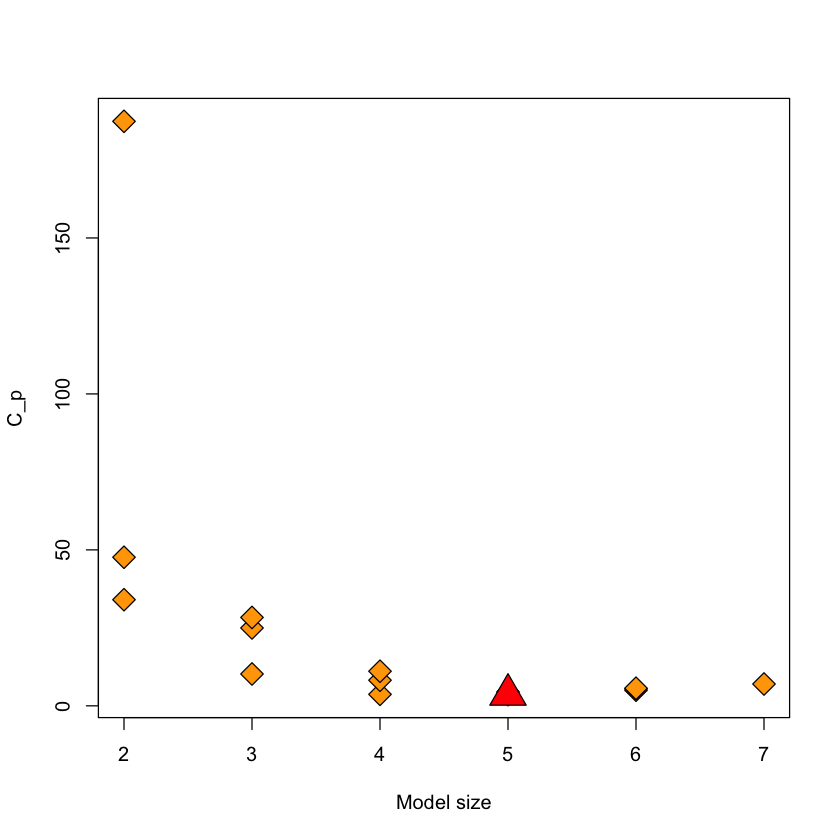
Figure

• Plot of \(C_p\) of a model as a function of the model size.

• The “best” model in terms of \(C_p\) is not the full model: has size 5 (4 variables plus intercept)

• Agrees with R^2_a.

Sequential search (step in R)

• The step function uses a specific score for comparing models.

Akaike Information Criterion (AIC)

\[AIC({\cal M}) = - 2 \log L({\cal M}) + 2 \cdot p({\cal M})\]

• Above, \(L({\cal M})\) is the maximized likelihood of the model.

Bayesian Information Criterion (BIC)

\[BIC({\cal M}) = - 2 \log L({\cal M}) + \log n \cdot p({\cal M})\]

• Note: AIC/BIC be used for whenever we have a likelihood, so this generalizes to many statistical models.

AIC for regression

• In linear regression with unknown \(\sigma^2\)

\[-2 \log L({\cal M}) = n \log(2\pi \widehat{\sigma}^2_{MLE}) + n\]

• In linear regression with known \(\sigma^2\)

\[-2 \log L({\cal M}) = \frac{1}{\sigma^2} SSE({\cal M})\]

• AIC is very much like Mallow’s \(C_p\) with known variance.

n = nrow(X_SAT)
p = length(coef(SAT.lm)) + 1
c(n * log(2*pi*sum(resid(SAT.lm)^2)/n) + n + 2*p, AIC(SAT.lm))

1. 477.477004344384
2. 477.477004344384

Properties of AIC / BIC

• BIC will typically choose a model as small or smaller than AIC (if using the same search direction).

• As our sample size grows, under some assumptions, it can be shown that

  1. AIC will (asymptotically) always choose a model that contains the true model, i.e. it won’t leave any variables out.

  2. BIC will (asymptotically) choose exactly the right model.

SAT example

Let’s take a look at step in action. Probably the simplest strategy is forward stepwise which tries to add one variable at a time, as long as it can find a resulting model whose AIC is better than its current position.

When it can make no further additions, it terminates.

SAT.step.forward = step(lm(SAT ~ 1, SAT.df), 
                        list(upper = SAT.lm),
                        direction='forward', 
                        trace=FALSE)
names(coef(SAT.step.forward))[-1]

1. 'Rank'
2. 'Years'
3. 'Expend'
4. 'Public'

Interactions and hierarchy

• Wildcard: . denotes any variable in SAT.df except SAT

• .^2 denotes all 2-way interactions

SAT2.lm = lm(SAT ~ .^2, SAT.df)
SAT2.step.forward = step(lm(SAT ~ 1, SAT.df), 
                        list(upper = SAT2.lm),
                        direction='forward', 
                        trace=FALSE)
names(coef(SAT2.step.forward))[-1]

1. 'Rank'
2. 'Years'
3. 'Expend'
4. 'Public'
5. 'Years:Expend'
6. 'Years:Public'
7. 'Rank:Public'

• Note: when looking at trace=TRUE we see that step does not include an interaction unless both main effects are already in the model.

BIC example

The only difference between AIC and BIC is the price paid per variable. This is the argument k to step. By default k=2 and for BIC we set k=log(n). If we set k=0 it will always add variables.

SAT.step.forward.BIC = step(lm(SAT ~ 1, SAT.df), 
                            list(upper=SAT.lm),
                            direction='forward', 
                            k=log(nrow(SAT.df)),
                            trace=FALSE)
names(coef(SAT.step.forward.BIC))[-1]

1. 'Rank'
2. 'Years'
3. 'Expend'

Compare to AIC

names(coef(SAT.step.forward))[-1]

1. 'Rank'
2. 'Years'
3. 'Expend'
4. 'Public'

Backward selection

Just for fun, let’s consider backwards stepwise. This starts at a full model and tries to delete variables.

There is also a direction="both" option.

SAT.step.backward = step(lm(SAT ~ ., SAT.df), 
                        list(lower = ~ 1),
                        direction='backward', 
                        trace=FALSE)
names(coef(SAT.step.backward))[-1]

1. 'Years'
2. 'Public'
3. 'Expend'
4. 'Rank'

Compare to forward

names(coef(SAT.step.forward))[-1]

1. 'Rank'
2. 'Years'
3. 'Expend'
4. 'Public'

Summarizing results

The model selected depends on the criterion used.

Criterion	Model
\(R^2\)	~ .
\(R^2_a\)	~ Years + Public + Expend + Rank
\(C_p\)	~ Years + Public + Expend + Rank
AIC forward	~ Years + Public + Expend + Rank
BIC forward	~ Years + Expend + Rank
AIC forward .^2	~ Years + Public + Expend + Rank + Years:Expend + Years:Public + Rank:Public

The selected model is random and depends on which method we use!

Pretty stable for this analysis.

Where we are so far

• Many other “criteria” have been proposed: cross-validation (CV) a very popular criterion.

• Some work well for some types of data, others for different data.

• Check diagnostics!

• These criteria (except cross-validation) are not “direct measures” of predictive power, though Mallow’s \(C_p\) is a step in this direction.

• \(C_p\) measures the quality of a model based on both bias and variance of the model. Why is this important?

• Bias-variance tradeoff is ubiquitous in statistics!

Case study B: sex discrimination

Possible goals in the salary data

• Interested in the effect of Sex but there could lots of other covariates we might adjust for…

• Considering all second order effects (besides Sex) in salary: \(2^{14}\) models!

• Remove confounders, reduce variability of Sex effect.

Approach

1. Fit a model without Sex using a model selection technique.

2. Estimate the effect of Sex by adding it to this model.

How are we going to choose \(2^{14}\) possible choices!

---

D = with(salary, cbind(Senior, Age, Educ, Exper))
base.lm = lm(Bsal ~ poly(D, 2), data=salary)
summary(base.lm)$coef

A matrix: 15 × 4 of type dbl

	Estimate	Std. Error	t value	Pr(>|t|)
(Intercept)	5582.2150	248.1313	22.4970203	7.638697e-36
poly(D, 2)1.0.0.0	-1573.9454	604.3710	-2.6042704	1.101964e-02
poly(D, 2)2.0.0.0	-557.6906	598.3874	-0.9319892	3.542180e-01
poly(D, 2)0.1.0.0	-3296.2869	1205.0112	-2.7354823	7.708189e-03
poly(D, 2)1.1.0.0	-1391.7057	10662.3569	-0.1305252	8.964870e-01
poly(D, 2)0.2.0.0	642.9167	1481.8206	0.4338695	6.655809e-01
poly(D, 2)0.0.1.0	2803.3752	624.6501	4.4879128	2.448263e-05
poly(D, 2)1.0.1.0	-8988.2242	5831.5630	-1.5413062	1.272897e-01
poly(D, 2)0.1.1.0	-13458.5332	10422.6307	-1.2912799	2.004204e-01
poly(D, 2)0.0.2.0	511.2407	617.2702	0.8282284	4.100682e-01
poly(D, 2)0.0.0.1	5148.9154	2440.3756	2.1098865	3.807450e-02
poly(D, 2)1.0.0.1	3111.7689	11658.6746	0.2669059	7.902460e-01
poly(D, 2)0.1.0.1	-22769.0399	27351.7731	-0.8324521	4.076954e-01
poly(D, 2)0.0.1.1	-5858.7426	9012.8843	-0.6500408	5.175758e-01
poly(D, 2)0.0.0.2	-671.2631	1646.9549	-0.4075783	6.846998e-01

Best second order model using \(C_p\) with leaps

X_sal = model.matrix(base.lm)[,-1]
Y_sal = log(salary$Bsal)
salary.leaps = leaps(X_sal, Y_sal, nbest=10, method='Cp')
Cp_idx = which((salary.leaps$Cp == min(salary.leaps$Cp)))
best.model.Cp = salary.leaps$which[Cp_idx,]
colnames(X_sal)[best.model.Cp]

1. 'poly(D, 2)1.0.0.0'
2. 'poly(D, 2)0.1.0.0'
3. 'poly(D, 2)0.0.1.0'
4. 'poly(D, 2)1.0.1.0'
5. 'poly(D, 2)0.1.1.0'
6. 'poly(D, 2)0.0.0.1'
7. 'poly(D, 2)0.1.0.1'

Plot of \(C_p\) scores (Fig 12.11 in book)

plot(salary.leaps$size,
     salary.leaps$Cp,
     pch=23,
     bg='orange',
     cex=2, 
     ylim=c(0, 15))
points(salary.leaps$size[Cp_idx],
       salary.leaps$Cp[Cp_idx],
       pch=24,
       bg='red',
       cex=3)

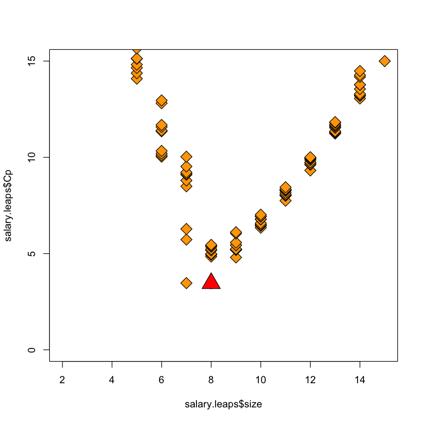
Figure:

• Plot of \(C_p\) score as a function of model size.

• Two models are lower than the rest but quite close. These models used in subsequent analysis.

Estimating the effect of Sex

summary(lm(log(Bsal) ~ Sex + X_sal[,best.model.Cp], data=salary))$coef['SexMale',]

Estimate

0.117337805016164

Std. Error

0.0229093663345294

t value

5.12182673683605

Pr(>|t|)

1.89648601842772e-06

• On inspection, book drops one of these interactions:

summary(lm(log(Bsal) ~ Sex + X_sal[,best.model.Cp][,-4], data=salary))$coef['SexMale',]

Estimate

0.119590116093162

Std. Error

0.0229149605616616

t value

5.21886632845638

Pr(>|t|)

1.25496659910706e-06

What if we used step?

step_df = with(salary, data.frame(Bsal, X_sal))
step_lm = lm(log(Bsal) ~ ., step_df)
step_sel = step(lm(log(Bsal) ~ 1, data=step_df),
                list(upper=step_lm),
		trace=FALSE)
names(coef(step_sel))[-1]

1. 'poly.D..2.0.0.1.0'
2. 'poly.D..2.1.0.0.0'
3. 'poly.D..2.0.1.1.0'
4. 'poly.D..2.0.0.0.1'
5. 'poly.D..2.0.1.0.0'
6. 'poly.D..2.0.1.0.1'
7. 'poly.D..2.1.0.1.0'

Larger example

• As \(p\) grows, leaps will be too slow

• Even step can get slow

HIV resistance

• Resistance of \(n=633\) different HIV+ viruses to drug 3TC.

• Features \(p=91\) are mutations in a part of the HIV virus, response is log fold change in vitro.

url_X = 'https://raw.githubusercontent.com/StanfordStatistics/stats191-data/main/NRTI_X.csv'
url_Y = 'https://raw.githubusercontent.com/StanfordStatistics/stats191-data/main/NRTI_Y.txt'
X_HIV = read.table(url_X, header=FALSE, sep=',')
Y_HIV = read.table(url_Y, header=FALSE, sep=',')
Y_HIV = as.matrix(Y_HIV)[,1]
X_HIV = as.matrix(X_HIV)
dim(X_HIV)

1. 633
2. 91

---

D = data.frame(X_HIV, Y_HIV)
M = lm(Y_HIV ~ ., data=D)
M0 = lm(Y_HIV ~ 1, data=D)
system.time(MF <- step(M0,
                 list(lower=M0,
		      upper=M), 
                 trace=FALSE,
		 direction='both'))
names(coef(MF))

   user  system elapsed 
  0.607   0.017   0.629 

1. '(Intercept)'
2. 'V68'
3. 'V17'
4. 'V19'
5. 'V23'
6. 'V54'
7. 'V67'
8. 'V82'
9. 'V32'
10. 'V81'
11. 'V87'
12. 'V57'
13. 'V41'
14. 'V31'
15. 'V29'
16. 'V30'
17. 'V70'
18. 'V39'
19. 'V26'
20. 'V69'
21. 'V40'
22. 'V62'
23. 'V64'
24. 'V80'

---

system.time(MB <- step(M,
                 list(lower=M0,
		      upper=M), 
                 trace=FALSE,
		 direction='both'))
names(coef(MB))		 

   user  system elapsed 
 12.363   0.132  12.674 

1. '(Intercept)'
2. 'V17'
3. 'V19'
4. 'V23'
5. 'V26'
6. 'V29'
7. 'V30'
8. 'V31'
9. 'V32'
10. 'V39'
11. 'V40'
12. 'V41'
13. 'V54'
14. 'V57'
15. 'V62'
16. 'V64'
17. 'V67'
18. 'V68'
19. 'V69'
20. 'V70'
21. 'V80'
22. 'V81'
23. 'V82'
24. 'V87'